

Translate this page into:
A new self-organization of complex networks structure generalized by a new class of fractional differential equations generated by 3D-gamma function
⁎Corresponding author. rabhaibrahim@yahoo.com (Rabha W. Ibrahim)
-
Received: ,
Accepted: ,
This article was originally published by Elsevier and was migrated to Scientific Scholar after the change of Publisher.
Abstract
In this note, we suggest a generalization of gamma function to be 3D-gamma function. As a consequence, some special functions are generalized including the Mittag–Leffler function. Moreover, we utilize the generalized Mittag–Leffler to extend the AB-fractional calculus. Examples are introduced to cover our theory. The solvability of abstract Riccati equation is considered, and Hyers–Ulam stability is discovered in the sequel. Based on the new study, we design new stable of Self-organization in complex networks (SOCNs).
Keywords
26A33
Gamma function
Generalized fractional calculus
Fractional differential operator
Mittag–Leffler function
Complex networks

1 Introduction
Numerous probability distributions, including the gamma distribution, chi-squared distribution, and exponential distribution, are strongly associated with the gamma function. Numerous statistical applications, such as theory of queues, reliability analysis, and delay modeling, include these distributions. An example of analytic continuation that permits its application to complex numbers is the gamma function. In complex analysis and the study of functions of a complex variable, this trait is crucial. Many branches of physics and engineering, such as quantum mechanics, fluid dynamics, electromagnetic, and signal processing, use the gamma function. It frequently comes up while defining answers to diverse physical issues and analyzing differential equations.
The gamma function, represented as
, is a real and complex number extension of the factorial function. In terms of positive integers, the factorial function and the gamma function are almost identical. It has been outlined nonetheless, for a considerably larger scope. It is defined by the integral
Relations of
are presented, as follows: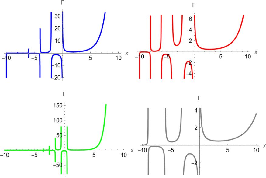
The plot of
when
and (2, 1, 3) accordingly.
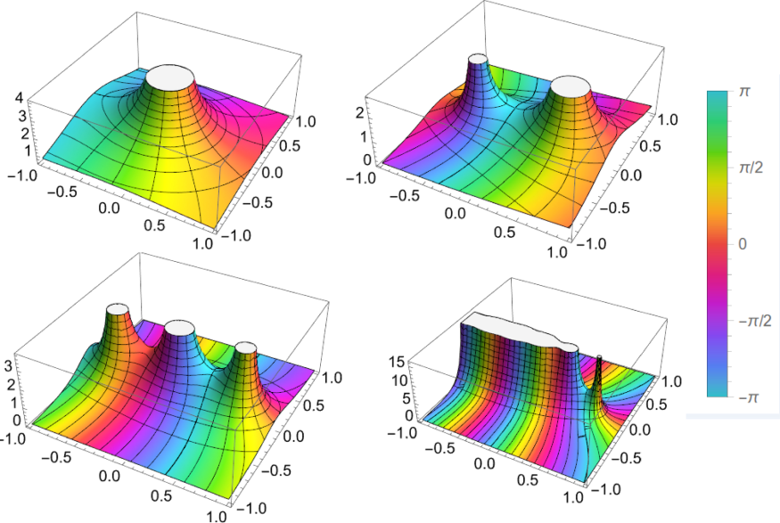
The ComplexPlot3D of
when
and (4, 3, 1) accordingly using Mathematica 14.1.
Let with , , and . Then
-
-
;
-
-
.
A direct application of the definition in (1.5) and using the asymptotic approximations of gamma function, we obtain the results. □
In view of , we generalize a set of special functions including the Mittag–Leffler function. As a consequence AB-fractional calculus is generated and discuss some of its properties, such as the boundedness. Applications based on the suggested model, the stability of self-organization in complex networks is investigated such that their dynamics and geometry change over time through decentralized processes.
2 3D-Mittag–Leffler functions (3D-MLFs)
Numerous branches of mathematics, such as probability theory, fractional calculus, and the theory of special functions, use this function. It may be used to describe complicated relaxation or waiting time behaviors in many phenomena. In the mathematical concept of fractional differential equations, it is important. In fractional calculus, a field of mathematics that extends the idea of differentiation and integration to non-integer orders, MLFs usually occur. They frequently show up as fractional differential equation solutions. They are used in the analysis of fractional differential equations regulating materials, anomalous transport processes, and fractional relaxing behaviors in the study of dynamical systems. The 2D-MLF is given by the description A generalization of this function is defined as follows: where Now, by using the generalized gamma function , we have and Clearly, when , and are reduced into and respectively. As a special case, when , we have (see Fig. 3)
Similarly for
, we have
where
is the normalized Fox–Wright function,
Next section deals with the generalization of AB-fractional calculus using the generalized 3D-Mittag–Leffler function.![The of [ Ξ a , b ] μ , ν , κ ( ξ ) = κ [ Ξ α κ , β κ ] ( ξ ) for different values, where κ = 1 , 2 , 3 , 4 respectively.](/content/185/2024/36/11/img/10.1016_j.jksus.2024.103512-fig3.png)
The of
for different values, where
respectively.
3 AB-fractional calculus
In Atangana and Baleanu (2016), Atangana and Baleanu presented a fractional calculus based on the Mittag–Leffler function, as follows: and where satisfies the relation , , is an interval, and Corresponding to the fractional derivatives, the fractional integral becomes Note that the above fractional operators are utilized in different applications (Abd-Elmonem et al., 2023; Momani et al., 2023; Ibrahim, 2022; Huang et al., 2023).
By using the suggested 3D-gamma function, we have Now, we introduce the following definitions.
Let and . Then the generalized AB-operators are as follows:
Note that when we obtain the usual . We have the following properties:
Let and be real numbers. Then for continuous functions and over , the generalized 3D-fractional operators satisfy the semi group property
-
;
-
;
-
.
Let . Then Let , , , and . Then Furthermore, we have Hence, we obtain Finally, we attain If then And if then Finally, suppose that . Then where indicates the incomplete Gamma function.
Assume that where . If and then
-
where and is the supremum norm;
-
.
-
.
By the definition of the suggested fractional operators, we have Moreover, we have Finally, we obtain
Consider the fractional differential equation
According to Proposition 3.4, we get Thus, a computation yields In other inequality, we have the result (3.2). □
Note that Eq. (3.1) represents the generalized Riccati equation, which will be considered as an application in the next section. Corollary 3.5 shows that the solution of Eq. (3.1) is bounded, with upper bound .
4 Suggested system of complex networks with solvability
The solvability of fractional differential equations is established by the subsequent theorems and the particular conditions of the equations. Various standards for evaluating these attributes may be applied to differential equation categorization. In this part, we deal with the solvability of the generalized fractional differential equation
For (4.1) (or (4.2)). If is bounded in its domain with then Eq. (4.1) admits a solution under the condition Moreover, if is a Lipschitz with respect to the second variable with then the solution is unique.
Consider Eq. (4.1). Define an operator such that by Thus, we obtain Hence, we obtain We obtain the boundedness of in the set , by choosing the supremum of the inequality mentioned earlier. Our goal is to demonstrate the continuity within . It is clear that Since is continuous then it is uniformly continuous in with As a consequence, we get This shows that is continuous over the set . We proceed to show that is equicontinuous over . Let and with . Thus, we get Thus, we obtain Hence, is a reasonably compact operator, as the Arzela–Ascoli theorem reveals. According to Schauder’s fixed point theorem, permits a minimum of one fixed point, which is analogous to the solvability of Eq. (4.1).
Next, we aim to show that the operator admits the unique fixed point over the set . Obviously, This implies that the operator is a contraction mapping over . Thus, according to Banach fixed point theorem, has one fixed point which is corresponding to the solution of Eq. (4.1). □
Consider the following equation:
Next, we consider the following fractional differential equation
5 Stability of the complex networks
In this section, we study the Ulam–Hyers stability (Hyers et al., 2012). There are different generalizations of the Ulam stability using the fractional calculus (see Ibrahim, 2012, 2013; Wang and Xu, 2015). Here, we aim to introduce another generalization, using the suggested fractional differential operators, as follows:
Consider Eq. (4.1). Then it is Ulam–Hyers stable if there occurs a real positive number
achieving the following conclusion: for all
and for every solution
,
Consider Eq. (4.1). Then it is Ulam–Hyers stable if there occurs a real positive number
satisfying the following conclusion: for all
and for every solution
,
Note that
is a solution of Eq. (4.1)if and only if there occurs a function
with
achieving the equation
Let the assumptions of Theorem 4.1 hold. Then Eq. (4.1) is a generalized Ulam–Hyers stable.
Assume that is a unique solution and a function such that and for a positive constant , we have Then a computation yields (see Box I)
that is where (see Theorem 4.1). Hence, Eq. (4.1) is a generalized Ulam–Hyers stable. □
Example 4.2 is generalized Ulam stability.
6 Applications on self-organization of complex networks
The concept of self-organization in complex networks is fascinating because it describes how separate components in the network interact to generate structured patterns or behaviors. One use of Riccati equations, which are frequently used in differential equations and control theory, is in the analysis of complex networks. In complex networks, the dynamics of the network’s connection or the growth of specific network properties can be simulated using Riccati equations (Peng et al., 2021; Klickstein et al., 2017). These equations could explain how one node interacts with the others or how the network topology changes over time. One way is to use Riccati equations to represent the dynamics of the network’s adjacency matrix, which displays the connections between nodes. The Riccati equations can describe the self-organizing behavior of the network by establishing appropriate rules for node interactions, which lead to the formation of specific designs or sequences. Additionally, Riccati equations may be used to study the stability and controllability of complex networks. By looking at the solutions to these equations, researchers can gain greater insight into how the structure of the network influences its overall behavior and usefulness. Generally speaking, using Riccati equations to analyze the behavior of complex networks provides a solid framework for understanding the self-organizing principles underlying the emergence of complex behaviors and trends in a range of systems, from biological networks to social networks and beyond (Duan et al., 2022; Vamvoudakis and Jagannathan, 2016). This study focuses on a multi-channel system in which an agent with network communication capabilities oversees every communication channel.
The particular dynamics system for the agent
is defined as follows (see Fig. 4):
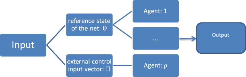
Block diagram showing a controller model that is referred to the suggested system (6.1).
-
The reference agent plays a crucial role in guiding the development, evaluation, and improvement of agents in a multi-agent system. A reference agent can serve as a benchmark or standard when comparing one agent to another. It might be an intelligently designed agent that demonstrates characteristics, methods, or behaviors deemed most optimal or appropriate for the specific task at hand or the environmental conditions. The approaches and activities of the reference agent may provide agents with hints and strategies. Through the analysis and assessment of the reference agent’s actions, other agents are able to improve and adjust their own processes for making decisions. The reference agent can be used as a model to set policies or criteria for agents’ behavior. By looking at how the reference agent behaves, designers might derive rules or guidelines that specify desired systemic behaviors.
-
A notepad that is used to play video games on a computer or console could be an example of an external controller. These controllers let players engage with games by pressing buttons, moving joysticks, or activating other input devices. They are usually connected to the gaming device wirelessly over Bluetooth or USB. Using an external controller instead of a keyboard and mouse allows for a more tactile and intuitive gaming experience.
7 Conclusion
From the above illustration, we have made a generalization for gamma function to get the 3D-gamma function. Based on this generalization, the Mittag–Leffler function is generalized. As a consequence, we considered 3D-AB-fractional calculus. Application is given for the generalized fractional Riccati equation. Examples are formulated using the suggested fractional operators. We considered the generalized Ulam stability for the solutions. We utilized the operator , which can be replaced by . Applications on self-organization of complex networks are proposed using the generalized fractional differential operators. For future efforts, we aim to make an extension of the suggested operators by using a complex analytic function of a complex variable. We constructed new stable SOCNs based on the recent studies. The optimal control is given in terms of the generalized Mittag–Leffler function.
CRediT authorship contribution statement
Ibtisam Aldawish: Visualization, Validation, Project administration, Funding acquisition. Rabha W. Ibrahim: Writing – review & editing, Writing – original draft, Software, Methodology, Investigation, Formal analysis.
Declaration of competing interest
The authors declare that they have no known competing financial interests or personal relationships that could have appeared to influence the work reported in this paper.
References
- A comprehensive review on fractional-order optimal control problem and its solution. Open Math.. 2023;21:20230105
- [Google Scholar]
- New fractional derivatives with nonlocal and non-singular kernel: theory and application to heat transfer model. Therm. Sci.. 2016;20(2):763-769.
- [Google Scholar]
- On hypergeometric functions and pochhammer K-symbol. Divulgaciones Matemticas. 2007;15:179-192.
- [Google Scholar]
- Self-organization cooperative output regulation. In: 2022 IEEE International Conference on Unmanned Systems. IEEE; 2022. p. :998-1003.
- [Google Scholar]
- Modified Atangana-Baleanu fractional operators involving generalized Mittag-Leffler function. Alex. Eng. J.. 2023;75:639-648.
- [Google Scholar]
- Stability of Functional Equations in Several Variables. Springer Science & Business Media; 2012.
- Ulam stability for fractional differential equation in complex domain. Abstr. Appl. Anal.. 2012;2012 Hindawi
- [Google Scholar]
- Ibrahim, Rabha W., 2022. Dumitru Baleanu Modified Atangana-Baleanu fractional differential operators. In: Proceedings of the Institute of Mathematics and Mechanics. vol. 22, pp. 1–12.
- Energy scaling of targeted optimal control of complex networks. Nat. Commun.. 2017;8(1):15145.
- [Google Scholar]
- K-symbol Atangana-Baleanu fractional operators in a complex domain. In: 2023 International Conference on Fractional Differentiation and Its Applications. IEEE; 2023. p. :1-4.
- [Google Scholar]
- Distributed extended state estimation for complex networks with nonlinear uncertainty. IEEE Trans. Neural Netw. Learn. Syst. 2021:1-9.
- [Google Scholar]
- New results on (r, k, )-Riemann–Liouville fractional operators in complex domain with applications. Fractal Fract.. 2024;8(3):165.
- [Google Scholar]
- Introduction to complex systems and feedback control. In: Control of Complex Systems. Butterworth-Heinemann; 2016. p. :3-30.
- [Google Scholar]
- Hyers-Ulam stability of fractional linear differential equations involving Caputo fractional derivatives. Appl. Math.. 2015;60(4):383-393.
- [Google Scholar]


