Thermocapillary effects on absolute and convective instability of viscoelastic liquid jets

1 Introduction

In liquid jets, the role of capillary thermodynamic effects on the (CI) and (AI) are still an open area of research and not well understood completely. (Bauer, 1984) was the first to examine the instability of non-isothermal jets (with temperature-dependent surface tension) by using linear stability theory. (Bauer, 1984) looked specifically at the case of the Stokes flow with adding temperature to the jet surface. He found that the jet can be broken up because of oscillating temperature gradients along the jet interface. (Xu and Davis, 1985) studied especially the linear axial distribution of temperature along the jet surface. They found that the capillary instability can be repressed, or obstructed by the instability of the surface wave produced by surface tension gradients. Whereas the first work in controlling the liquid jet disintegration was carried out by (Faidley and Panton, 1990) using a quick-response nozzle heater to control surface tension. They found that the Rayleigh mode was dominant and that the thermal effects were unimportant to the growth of the disturbances. However, by using a ${\mathit{CO}}_2$ laser beam with sufficient intensity, (Nahas and Panton, 1990) were able to demonstrate that it could be eliminated the initial turbulence on the jet surface, which indicates that the heater utilized by (Faidley and Panton, 1990) was not able to generate adequate nozzle heating.

The instability and following disintegration of the liquid jet column is important in a variety of emerging applications (for example, needleless injection (see Moradiafrapoli and Marston, 2017), nanofiber (see Gadkari, 2017), ink-jet printing (see Du et al., 2018), coating, and even technology of diesel engine (see Eggers and Villermaux, 2008). Although more than 200 years passed of scientific scrutiny, liquid jet instability is still an interesting area of study for many researchers in various scientific fields. A liquid jet may be defined as a stream that can be injected into a medium of liquid or gas through an opening (a nozzle). Liquid jets, in general, are naturally unstable and eventually disintegrated into drops. The Rayleigh-Plateau instability is the main mechanism of this dissociation and determined by the growth of perturbations that are either convective or absolute instability. Convective instability can be growing in amplitude when it is swept along by the liquid flow, while absolute instability can occur at particular spatial positions (see Bassi, 2011). Moreover, the formation of the droplet occurs either directly at the jet’s outlet or downstream, at the flow’s end. Jetting and dripping are the terms used to describe these two instabilities respectively (see Suñol and González-Cinca, 2015).

The first investigation of absolute instability related to liquid jets was done by (Leib and Goldstein, 1986b). They revealed that the capillary absolute instability of an inviscid jet is generated at small Weber numbers because of surface tension. They identified critical Weber numbers (We) that indicate the transition from (CI) to (AI). They showed that when the Weber number is less than $3.15$ , the inviscid liquid jet is absolutely unstable; whereas it is convectively unstable when $\mathit{We}>3.15$ . (Leib and Goldstein, 1986a) examined the viscosity effect on the transition from (CI) to (AI) and found a decrease in values of critical Weber number when We is a function of Re (where Re is the Reynolds number). Using the $\mathit{Re}-\mathit{We}$ plane, they plotted the relationship between Re and We numbers and discovered a crucial curve that distinguishes the area between absolute and convective instability. A criterion for analyzing absolute instability developed by (Briggs, 1964) was used by (Lin and Lian, 1989) to find the transition boundary between (CI) and (AI) for a viscous liquid in the presence of a surrounding gas. (Alhushaybari and Uddin, 2019) investigated the (CI) and (AI) of a viscoelastic liquid jet falling vertically due to gravity. They showed the convective/absolute instability boundaries (CAIB) in different parameter regimes and especially compared the (CAIB) in the $\mathit{Re}-\mathit{We}$ plane with other authors investigated the viscous case such as (Lin and Lian, 1989; Lin and Lian, 1993; Leib and Goldstein, 1986a and López-Herrera et al., 2010).

Nowadays, the instability for a liquid jet having complex rheology is significant in various emerging and growing applications (such as needle-free injections and fiber spinning where the jet stability is a prerequisite for the formation of fibers with desirable properties or successful injection (i.e. skin breakthrough) (see Moradiafrapoli and Marston, 2017). The instability of viscoelastic liquid jets also has some important applications in geodynamic fields related to underground mechanical explosions and earthquakes (see (Sharma et al., 2020; Pramanik and Manna, 2022 and Manna et al., 2018)). In these and other applications, the fluid utilized predominately contains additional quantities or biological agents that lead to the appearance of viscoelastic properties, and where instability is not desirable and the use of heating provides a technique for reducing the growth rates of unstable waves along the interface. In these applications, the use of heating provides one mechanism by which the growth of instability can be delayed. In light of this, this article investigates the absolute instability of a viscoelastic jet that is heated up at the nozzle and falls under gravity. We employ a mapping technique dubbed the ’Cusp Map Method’ developed by (Kupfer et al., 1987) to locate the cusp point corresponding to the pinch point, which indicates the transition of convective-to-absolute instability.

2 Problem formulation

Consider an axisymmetrical viscoelastic jet has radius a, surface tension $\sigma$ , thermal conductivity $k_t$ , temperature H, density $\rho$ , heat capacity $C_p$ and mean velocity U, which emerges from a nozzle, and falls under gravity into a surrounding of an inviscid gas, which has lower temperature $H_a$ and density ${\rho }_a$ . The jet leaving the nozzle is heated by a heater, which is connected to a computer so that the heating can be done in a controlled manner with a convenient frequency. To consider the axial symmetry problem, we suppose that the jet cross-section is remains circular $(\frac{\partial }{\partial \theta }=0)$ , and no swirl occurs $(v_{\theta }=0)$ , so the velocity vector is $\mathbf{v}$ $=(v_r,0,v_z)$ . The boundary conditions, as well as the governing equations, will be written in a cylindrical coordinate system where the z-axis runs parallel axis to the direction of the flow, whereas the r-axis runs perpendicular to the z-axis as depicted in Fig. 1.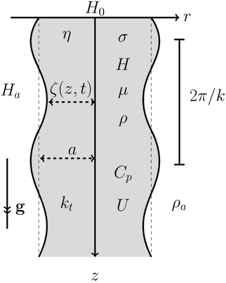

Close

Fig. 1

A diagram of a viscoelastic liquid jet emerging from a nozzle with computer-controlled heating.

Export to PPT

In viscoelastic fluids, the relation between stress and strain can be expressed by the Upper-Convected Maxwell model (see Bird et al., 1987), which is

At the jet interface, the boundary conditions are assessed by comparing the pressure across the free surface to the normal stresses, which are linked to the mean curvature by the relationship

3 Dimensionless analysis

Non-dimensionless scales used to write the dimensionless versions of the governing and boundary equations are (see Anno, 1977)

4 Asymptotic analysis

Following (Eggers, 1997), we give the jet a small aspect ratio ( $∊=a/L\ll 1$ ) by assuming that it is slender. These dimensionless equations (in Appendix A) are investigated in further details, so $v_z,v_r,p$ and H are expanded in a Taylor series in $∊r$ ; and $\zeta ,\mu ,T_{\mathit{zz}}$ and $T_{\mathit{rr}}$ are expanded in an asymptotic series in $∊$ . Also, we assume that small disturbances have no effect on the viscoelastic jet column’s centerline. Since $\zeta \left(z\right)$ changes slowly with respect to z (in the long wave limit), thus the pressure (p), the axial velocity ( $v_z$ ), and the components of the stress tensor ( $T_{\mathit{rr}}$ and $T_{\mathit{zz}}$ ) are nearly uniform with respect to r whilst $T_{\mathit{rz}}$ is roughly zero. As a result, a Taylor expansion of r is the appropriate ansatz for analyzing slender viscoelastic jets, which means that we have

To maintain viscoelastic and gravitational terms, we rescale the Reynolds and Froude numbers as follows: $\mathit{Re}=∊\widetilde{\mathit{Re}}=O\left(1\right)$ and $∊F^2=\widetilde{F^2}=O\left(1\right)$ (see Uddin, 2007). We substitute the expressions, (15) and (16), into the dimensionless forms (in Appendix A) and removing the tildes for simplicity, we can write the axial momentum equation, to $O\left(∊\right)$ , as

The kinematic boundary condition, (A.11), can be written, to leading order, as

5 Solutions of steady basic flow

In order to find steady basics flow solutions of (17)–(23), we first remove all time derivatives and then solve a nonlinear equations system, which has the four variables $T_{\mathit{rr}}^0,v_{z0},T_{\mathit{zz}}^0$ and $H_0$ as functions of z. Also, we find from (23) that $v_{z0}{\zeta }_0^2$ is constant, and using the boundary conditions at the nozzle ( $v_{z0}\left(0\right)=1$ and ${\zeta }_0\left(0\right)=1$ ) lead to have that $v_{z0}{\zeta }_0^2=1$ , and consequently the Eqs. (17)–(19) and (22) become respectively

The nonlinear system of ordinary differential equations, (24)–(27), are solved using the Runge–Kutta method (found in MATLAB ( $\mathit{ode}45$ )). Fig. 2 shows the gravity effect (through Froude’s different numbers F) on steady basic flow solutions ( $T_{\mathit{rr}}^0,T_{\mathit{zz}}^0,{\zeta }_0,v_{z0}$ and $H_0$ ) against the axial length of the jet (z) with and without heating. Solid lines show the solutions of the steady basic flow without heating; while dotted lines are the corresponding solutions with heating. We can see, from this figure, that a reduction in F accelerates the jet’s thinning and axial velocity increases. The inclusion of heating leads to an increase in the steady velocity along the viscoelastic jet leading to a faster decay in the radius of the jet along the z-direction of the jet. This is a consequence of the fact that the initial heating value $H_0$ decreases along the jet (see Fig. 2)(c) and, as a result, the surface tension increases with distance from the nozzle (the surface tension does, in fact, increase monotonically along the viscoelastic jet). We can see from Fig. 2 that this variation in surface tension causes a Marangoni flow to be induced along the jet axis. Because this flow operates in the direction of rising surface tension, the jet will accelerate toward the direction of gravity as a result. We conclude, from this result, that the heat energy transfer along the jet causes a Marangoni-type flow, that helps to make the jet thinner, leading to shorter lengths of breakup. We also can be seen that the steady axial tensor ( $T_{\mathit{zz}}^0$ ) of the viscoelastic liquid jet decreases with heating along the flow direction, whilst the steady radial tensor ( $T_{\mathit{rr}}^0$ ) increases. Moreover, we can also notice that increasing F leads to a decrease in ( $T_{\mathit{zz}}^0$ ) and an increase in ( $T_{\mathit{rr}}^0$ ) along the flow direction.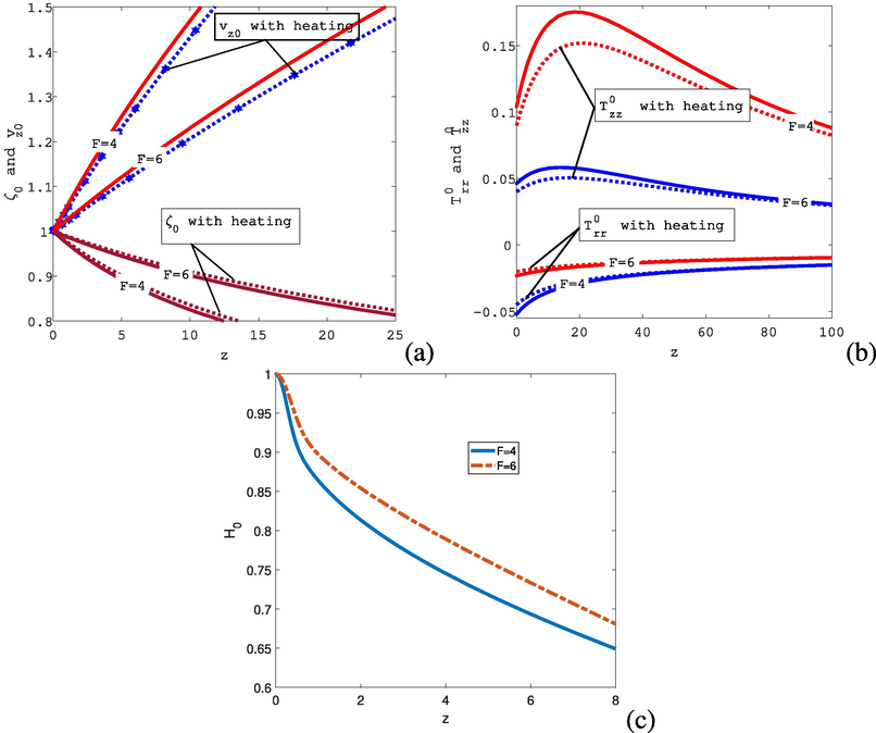

Close

Fig. 2

$v_{z0},{\zeta }_0,T_{\mathit{zz}}^0$ $T_{\mathit{rr}}^0$ and $H_0$ are plotted as a function of z for various values of F, where the solid lines in (a) and (b) show the steady basic solutions without heating (published by (Alhushaybari and Uddin, 2019)) with ${\mu }_H=H_0={\sigma }_H=0$ ), and the dotted lines in (a) and (b) show the steady basic solutions with heating (current work with ${\mu }_H=0.2,H_0=2$ and ${\sigma }_H=0.1$ ). Where $\mathit{De}=10,\mathit{Re}=800,\mathit{Pe}=10,\mathit{Bi}=0.2\text{.}$ and $\mathit{We}=2$ .

Export to PPT

6 Analysis of linear instability

Over an axial length scale of $z=O\left(1\right)$ , the viscoelastic jet develops. But, waves (having wavelengths of $O\left(a\right)$ ) are much smaller along the viscoelastic jet, that are analogous to $∊$ in a scenario where $z=O\left(1\right)$ is present. This multiscale technique was utilized by (Uddin, 2007). We use $\mathit{exp}(\mathit{ik}\overline{z}+\omega \overline{t})$ as a model for the traveling wave mode, where $t=∊\overline{t},z=∊\overline{z},k=k\left(z\right)=O\left(1\right)$ and $\omega =\omega \left(z\right)=O\left(1\right)$ . We use the following substitutions to apply a small perturbation about the solutions of the steady basic flow, which are

7 Convective instability analysis

The convective instability analysis includes two different instability analyses: temporal instability analysis, where it requires real wavenumber and complex frequency, and spatial instability analysis, where it requires the wavenumber to be complex and the frequency to be purely imaginary.

7.1

7.1 Temporal instability analysis

In the dispersion relation, (32), we consider k as a real wavenumber and $\omega$ as a complex frequency, where ${\omega }_i$ is $2\pi$ times frequency of the perturbation and ${\omega }_r$ is the perturbation growth rate. Then the Newton–Raphson method is utilized to solve this relation. Solving this dispersion relation yields the wavenumber corresponding to the greatest value of $\mathit{Re}\left(\omega \right)$ , which is the highest unstable wavenumber. The values of the steady basic flow vary with z, so the related wavenumber will also vary (see Section 5), therefore the corresponding growth rate will also change downstream (see Uddin, 2007).

The relation between $\mathit{Re}\left(\omega \right)$ and k is plotted, for two different Peclet numbers, as depicted in Fig. 3(a). From this figure, we see that when the Peclet number is decreased (which corresponds to a stronger influence of thermal diffusion over inertia), the growth rate drops and jets become longer. Also we can see that the highest unstable wavenumber is increased by increasing the Peclet number. The highest unstable wavenumber can be thought of as an inverse standard (by wavelengths) of the expected droplet sizes. In this consideration, Fig. 3(a) indicates that increasing the Peclet number will result in shorter jets as well as reduced droplet sizes. In Fig. 3(b) the temporal growth rate for various values of the Biot number is plotted. We note, from this figure, that the growth rate decreases as the Biot number increases. Also, we plot the relation between $\mathit{Re}\left(\omega \right)$ and k, for four different values of ${\mu }_H$ , as depicted in Fig. 3(c). As illustrated in this figure, the growth rate decreases as the value of ${\mu }_H$ increases. Additionally, we plot the relationship between $\mathit{Re}\left(\omega \right)$ and k for various values of ${\sigma }_H$ in Fig. 3(d). We find that increasing the value of ${\sigma }_H$ results in a decrease in the growth rate, as illustrated in this figure. Thus we might expect that viscoelastic jets will be longer with heating (because of the reduced growth rate of the perturbation) with larger drops (because of greater wavelengths corresponding to the faster-growing mode). Furthermore, from Fig. 3(b), we note that an increase in the Biot number reduces the range of instability (that is, the range of k values that causes growth in the waves). These results are in line with observations by (Uddin, 2007) for viscous liquid jets with heating.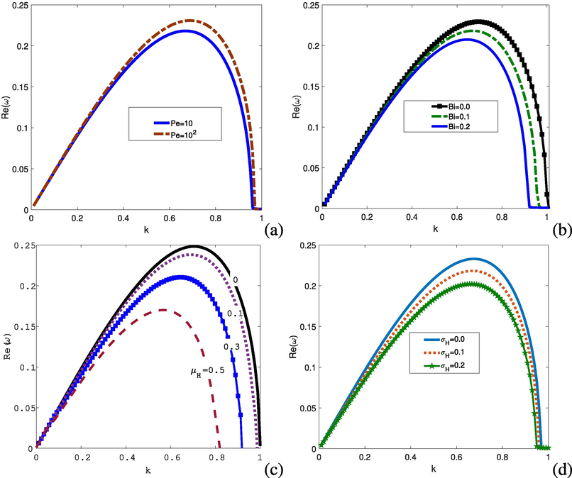

Close

Fig. 3

${\omega }_r$ against k for different values of $\mathit{Pe},\mathit{Bi},{\mu }_H$ and ${\sigma }_H$ respectively. Where $F=4,\mathit{Re}=800$ and $\mathit{De}=10$ at $z=0$ .

Export to PPT

7.2

7.2 Spatial instability analysis

A spatial instability analysis proposed by (Keller et al., 1973) is a more physically realistic analysis of the investigation of a liquid jet instability spatially, where disturbances grow in space rather than with time. This analysis assumed to set k as a complex wavenumber and $\omega$ as an imaginary frequency. Therefore, the spatial instability may be better in describing the physical process of the jet disintegration (see Busker et al., 1989). Spatial instability is also used in simulating satellites that form before or after the formation of the main droplets based on the amplitude of the disturbance. Comparison of theoretical foretelling and experimental findings carried out by (Si et al., 2009) points out that spatial instability results are in line with experiments better than temporal instability analysis, especially for medium to large Weber numbers (see Xie et al., 2017).

Following (Keller et al., 1973), in the dispersion relation (32), we consider k as a complex wavenumber and $\omega$ as a real frequency, where $\mathit{Im}\left(k\right)$ is the spatial perturbation growth rate. For unstable perturbations, we need $\mathit{Im}\left(k\right)<0$ since the most negative value of $\mathit{Im}\left(k\right)$ gives the largest spatial growth rate. We use the numerical method of Newton–Raphson to solve this dispersion relation for k together with given values of $\omega$ . We plot the relation between $\mathit{Re}\left(k\right)$ and $\mathit{Im}\left(k\right)$ for different values of Pe and Bi as depicted in Fig. 4a) and Fig. 4(b) respectively. We notice from Fig. 4(a) that the spatial growth rate is decreased when the Peclet number is decreased. While we notice from Fig. 4(b) that the spatial growth rate is decreased by increasing the values of the Biot number, which means that connecting heating to the free surface of the viscoelastic jet results in longer breakup lengths (i.e. heating has a stabilizing effect on the disintegration of the viscoelastic jet). Also, we observe from Fig. 4a) and Fig. 4(b) that the range of instability (i.e., values of $k_r$ at which the viscoelastic jet is unstable) is affected, where the inclusion of heating leads to a reduction in this range of instability. Also, we plot the relation between $\mathit{Re}\left(\omega \right)$ and $\mathit{Im}\left(\omega \right)$ , for three different values of ${\sigma }_H$ , as depicted in Fig. 4(c). As illustrated in this figure, the spatial growth rate decreases as the value of ${\sigma }_H$ decreases. Additionally, we plot the relationship between $\mathit{Re}\left(\omega \right)$ and $\mathit{Im}\left(\omega \right)$ for various values of ${\mu }_H$ in Fig. 4(d). We find that increasing the value of ${\mu }_H$ results in a decrease in the spatial growth rate, as illustrated in this figure.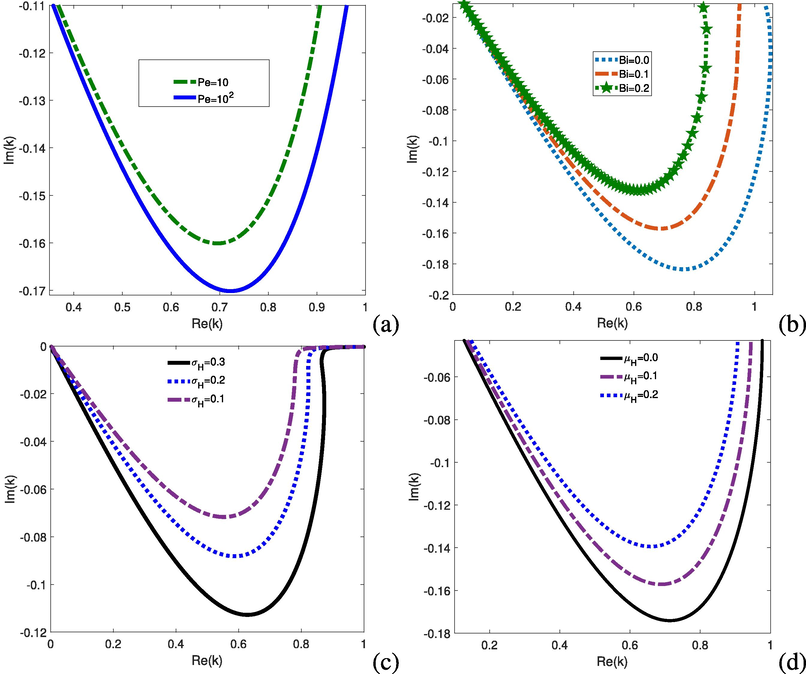

Close

Fig. 4

The graph illustrates the relationship between $\mathit{Im}\left(k\right)$ and $\mathit{Re}\left(k\right)$ for various values of $\mathit{Pe},\mathit{Bi},{\mu }_H$ and ${\sigma }_H$ respectively. Where $\mathit{De}=10,\mathit{We}=2,F=4$ and $\mathit{Re}=800$ at $z=0$ .

Export to PPT

8 Absolute instability analysis

Depending on the wave packets’ movement that growing along the viscoelastic jet, there are two different kinds of instability. We say that the flow is absolute instability when entire wave packets move up or down and there are time-dependent perturbations that grow at every fixed spatial point. If not, the flow could be convective instability, which grows and spreads far from its point of origin. This gives rise to the viscoelastic jet rupturing elsewhere away from the origin and leaving the jet to be unaffected at this origin (see Drazin and Reid, 1981). In turn, absolute instability spreads far from its origin point; however, it destabilizes the viscoelastic jet everywhere, including at the point of origin of the disturbance. For absolute instability, following (Briggs, 1964) criterion, we take a wave mode $\mathit{exp}(\omega t+\mathit{ikz})$ , where $\omega$ and k are both complex. Therefore, absolute instability takes place if the solution of (32) is found in the complex k-plane. This solution is called a saddle point corresponding to a cusp point (a pinch point) in the complex $\omega$ -plane.

When two $k\left(\omega \right)$ curves in the complex-frequency plane intersect, it forms a ”cusp point”. Absolute instability necessitates a $\mathit{Re}\left(\omega \right)>0$ dispersion relation solution. Confirmation of absolute instability occurs when the group velocity (given by a $\partial \omega /\partial k$ ) is 0 at the $k_0$ saddle point (which is a necessary condition, but not a sufficient one). This is due to the fact that the group velocity is not just zero in saddle points, but also at the convergence of two k branches regardless of whether or not the branches came from the same plane representing the half-k. To address this, a mapping procedure is created by (Kupfer et al., 1987), where pinch points are discovered by mapping selected contour lines from the $(k_r-k_i)$ -plane into the $({\omega }_r-{\omega }_i)$ -plane. When these lines are deformed, a branch point termed a cusp point appears in the $\omega$ -plane. Simultaneously, a pinch point emerges in the $(k_r-k_i)$ -plane. Additional distortions of contour lines after the establishment of the pinch point violate causality, and these deformations are halted. The following procedure can be used to determine whether or not the cusp point was formed by the k-branches created from two various halves of the $(k_r-k_i)$ -plane. As stated by (Kupfer et al., 1987), one can determine whether or not a pinch point exists at a cusp point by drawing a straight beam (parallel to the $\mathit{Re}\left({\omega }_r\right)$ -axis) starting from the cusp point and finishing with the first contour image (for $k_i=0$ ) and counting the intersections at which the beam intersects this image. If the number of the intersections is odd, then we are sure that the cusp point was formed by two various k-branches originating from two separate half of the $(k_r-k_i)$ -plane, and it is known as a pinch point.

8.1

8.1 Discovering the cusp point

(Kupfer et al., 1987) are shown that a $D(\omega ,k)=0$ dispersion relation may identify absolute instability from mapping the complex-frequency plane to the wavenumber plane. However, for a large number of physical techniques, the dispersion relation is used as a polynomial in $\omega$ rather than a transcendental in k. Solving for $\omega$ given a k is easier than solving for k given a $\omega$ . Because it is simpler to map from the $(k_r-k_i)$ -plane to the frequency plane than it is to solve transcendental equations (i.e. we can determine stability characteristics without having to solve them). The image of the region in the $(k_r-k_i)$ -plane is bounded on one side by the first contour created by mapping the complex wavenumber plane’s real line. Numerous contour lines exist throughout the range of unstable wavenumbers. If the contour lines are mapped into the $({\omega }_r-{\omega }_i)$ -plane, each contour line terminates in this specific area and leaves its image. A cusp point may be formed by constant parallel beams $\mathit{Im}\left(k\right)<0$ mapped on the $({\omega }_r-{\omega }_i)$ -plane. Assuming that a cusp point can be identified, it will correspond to the complex frequency plane value ${\omega }_0$ in the $({\omega }_r-{\omega }_i)$ -plane. This point is generated in the complex wavenumber plane by an associated value of $k=k_0$ . We have $\partial D({\omega }_0,k_0)/\partial k=0$ and $D({\omega }_0,k_0)=0$ by definition. Pinch point is identified when ${\omega }_0$ and $k_0$ are such that ${\partial }^{2}D({\omega }_0,k_0)/\partial k^2\ne 0$ . Thus, $\omega ={\omega }_0$ denotes the cusp point’s position in the $({\omega }_r-{\omega }_i)$ -plane, whereas $k\left({\omega }_0\right)$ denotes the saddle point’s position in the $k$ –plane corresponding to the cusp point ${\omega }_0$ . One can conclude that the relationship, ${(k-k_0)}^2\sim \omega -{\omega }_0$ , is a basic characteristic of forming the branching point (the cusp point) in the complex $\omega$ -plane, depending on whether the pinch point in the $(k_r-k_i)$ -plane is a saddle point or not. To search the cusp point, search the plane of k through $k_r$ -contour lines with different $k_i<0$ values and plot the contour lines images in the complex $\omega$ -plane. When the contour lines are close to the singularity, these images of the contour lines form a cusp. A contour line with the exact cusp point ( ${\omega }_0$ ) will appear on one of these contour lines. Once the cusp point is determined, the sign of ${\omega }_0$ can be used to identify the type of instability (convective or absolute). The flow of the liquid jet is absolutely unstable if ${\omega }_{0r}>0$ , and convectively unstable if ${\omega }_{0r}<0$ ; otherwise, the flow is stable (see Li et al., 2019).

Cusp map method does not depend on any mathematical formulae to determine where a cusp should be placed. Rather than that, we consider mappings of our k contours onto the frequency plane (varying real part, fixed imaginary part). This results in a curve that frequently loops back on itself. Therefore, following the idea of the cusp map method by looking at line mappings with $\mathit{Im}\left(k\right)=k_i$ (constant) in the $(k_r-k_i)$ -plane on the $({\omega }_r-{\omega }_i)$ -plane is referred to as the cusp curve, which is a set of points. Applying this method, if $k_i=0$ and keep changing $k_r$ -values yields the image of 1st contour of the dispersion relation, which corresponds to the largest growth rate of the temporal instability, as depicted in Fig. 3(a) when $\mathit{Pe}=10$ (the blue one). When $k_i$ values are reduced to negative values, we obtain the corresponding images of the dispersion relation, (32), in the $({\omega }_r-{\omega }_i)$ -plane as depicted in Fig. 5(a). If $k_i=-0.2$ , we observe that the cusp point appears at ${\omega }_0=0.068-0.81i$ , which corresponds to the $k_0$ (the saddle point) in the $(k_r-k_i)$ -plane. This is called a pinch point because when we draw a straight beam parallel to the $\mathit{Re}\left(\omega \right)$ -axis from it to the image of the 1st $k_r$ -contour line (for $k_i=0$ ) in the $({\omega }_r-{\omega }_i)$ -plane, there is only a point of intersection (odd number) (see (Patne and Shankar, 2017; Camporeale et al., 2017). In Fig. 5(a), the flow is absolutely unstable due to the fact that ${\omega }_{0r}>0$ .

Close

Fig. 5

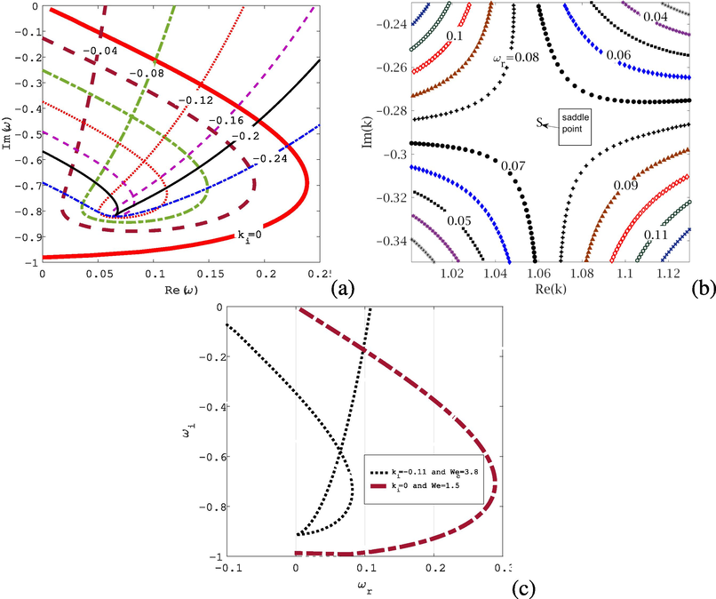
Graph (a) illustrating the $k_r$ -contour for various $k_i$ values in the $({\omega }_r-{\omega }_i)$ plane. The black line represents the cusp curve (when $k_i=-0.2$ ), contains the cusp point, whereas the red thick line represents the 1st $k_r$ -contour (when $k_i=0$ ). Graph (b) illustrating the saddle point, which is located in the complex k-plane at $k_0=1.062-0.288i$ , between 2 spatial branches of $\mathit{Im}\left(\omega \right)$ contour (when $\mathit{Re}\left(\omega \right)=0.07$ and ${\omega }_r=0.08$ respectively). Graph (c) shows the cusp point movement in the complex $\omega$ plane. When $\mathit{We}=1.5$ , the think red dashed line is the first contour line (for $k_i=0$ ); while the blue line is the cusp curve (for $k_i=-0.11$ ), which indicates the transition from (AI) to (CI) at $\mathit{We}={\mathit{We}}_c=3.8$ . Other parameters are $\mathit{De}=10,\mathit{Pe}=10,\mathit{Bi}=0.2,F=4,{\mu }_H=0.2,{\sigma }_H=0.1$ and $\mathit{Re}=800$ at $z=0$ .

Export to PPT

8.3

8.3 Discovering the CAIB

In order to locate the CAIB (convective-absolute instability boundary), we must monitor the cusp point as the Weber number is increased and all other dimensionless parameters are held fixed. We then find $\omega$ values at the cusp point using the Newton–Raphson method. This procedure is repeated until the Weber number reaches a critical value (that is, when the sign of ${\omega }_r$ changes from negative to positive), the critical value of $\mathit{We}={\mathit{We}}_c$ at which the transition occurs from absolutely unstable to convectively unstable, i.e. ${\omega }_{0r}=0$ ), as depicted in Fig. 5(c). In this case, the critical value of We (i.e., ${\mathit{We}}_c$ ) will be used to identify the convective/absolute instability boundary (CAIB), which will be the boundary between the convective and absolute regions (see Mohamed et al., 2015; Li et al., 2011). The same procedure is followed for various values of Re in the $(\mathit{Re}-\mathit{We})$ -plane, as depicted in Fig. 6(a), and in the $(\mathit{We}-\mathit{De})$ -plane, as depicted in Fig. 6(b), where ${\mathit{We}}_c$ denotes the location of the CAIB. Finally, in Fig. 7(a), the CAIB is identified by ${\mathit{We}}_c$ values, with different values of Bi, in the $(\mathit{We}-\mathit{Bi})$ -plane using the same process above.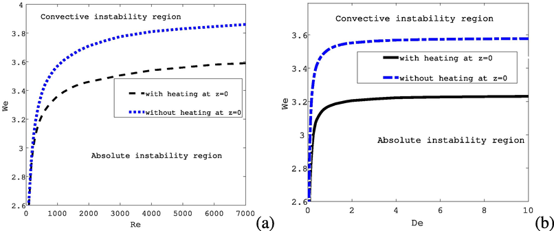

Close

Fig. 6

On the Re-We plane, a graph (a) depicting the convective/absolute instability boundary (CAIB) emerges at ${\omega }_r=0$ . While, on the De-We plane, a graph (b) depicting the convective/absolute instability boundary (CAIB) emerges at ${\omega }_r=0$ . Where $F=4,\mathit{Pe}=10,\mathit{Bi}=0.2,{\mu }_H=0.2,{\sigma }_H=0.1$ at $z=0$ .

Export to PPT

Close

Fig. 7

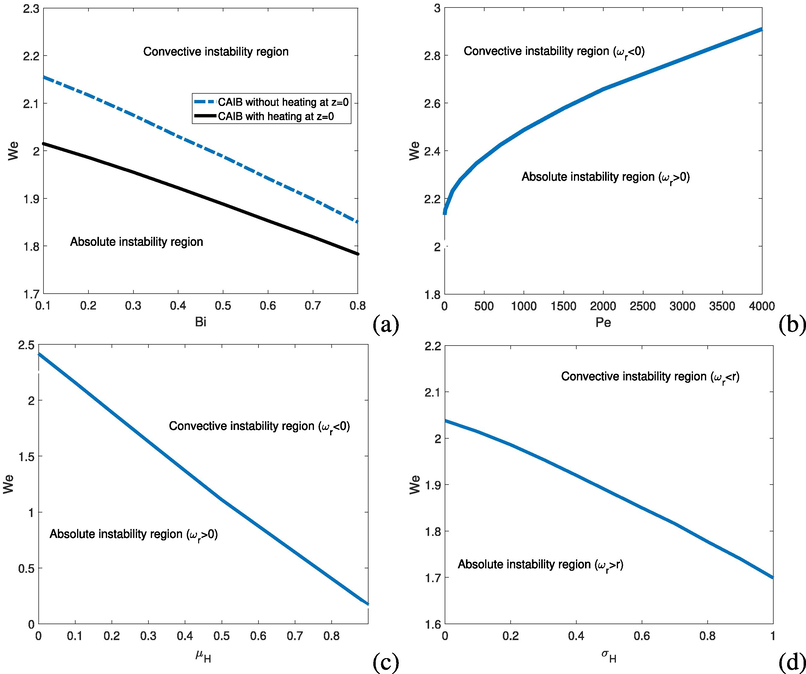
On the Bi-We plane, a graph (a) depicting the convective/absolute instability boundary (CAIB) emerges at ${\omega }_r=0$ . On the Pe-We plane, a graph (b) depicting the convective/absolute instability boundary (CAIB) emerges at ${\omega }_r=0$ . On the ${\mu }_H$ -We plane, a graph (c) depicting the convective/absolute instability boundary (CAIB) emerges at ${\omega }_r=0$ . On the ${\sigma }_H$ -We plane, a graph (d) depicting the convective/absolute instability boundary (CAIB) emerges at ${\omega }_r=0$ . Where $\mathit{Re}=800,\mathit{De}=10,F=4$ at $z=0$ .

Export to PPT

Also, in Fig. 6(a), we observe that when the viscosity reduces (by increasing Re values), the CAIB increases (i.e. an increase in ${\mathit{We}}_c$ values), where the CAIB increases abruptly in the range ( $500>\mathit{Re}>0$ ), and then rises progressively when $\mathit{Re}>500$ , indicating a delay in the transition from absolute to convective instability. According to its qualitative behavior, the CAIB is similar to that observed in (López-Herrera et al., 2010; Lin and Lian, 1989; Lin and Lian, 1993). Additionally, we observe that the inclusion of heating decreases ${\mathit{We}}_c$ values for various values of Re. In addition, we can see from this figure that the inclusion of heating has resulted in a smaller region of absolute instability being observed. In a similar way to gravitational forces, the Marangoni-induced flow, which works in the direction of gravity, acts in the opposite direction of wave propagation, preventing it from propagating upstream. Fig. 6(b) shows a sharp rise in CAIB ( $1>\mathit{De}>0$ ) and then asymptotes, which shows that the highest value of ${\mathit{We}}_c$ is $3.6$ without heating, while the largest value of ${\mathit{We}}_c$ is $3.22$ with heating. In Fig. 7(a), the CAIB (i.e. the critical Weber number) decreases as the Biot number rises, implying that the flow is absolutely unstable when both the Weber and Biot numbers are simultaneously decreased. Additionally, we observe that the maximum value of ${\mathit{We}}_c$ decreases with heating. Moreover, we plot the CAIB on the $\mathit{Pe}-\mathit{We}$ plane as depicted in Fig. 7(b). We note, from this figure, that the critical Weber number ( ${\mathit{We}}_c$ ) increases as the Peclet number increases. While the critical Weber number is decreased by increasing the value of ${\mu }_H$ as depicted in Fig. 7(c). Also, increasing the value of ${\sigma }_H$ leads to a decrease in ${\mathit{We}}_c$ as illustrated in Fig. 7(d).

9 Conclusion

This paper has looked into the (CI) and (AI) of a viscoelastic liquid jet that has fallen under the influence of gravity. We have used the UCM model and obtained steady basic flow solutions using an asymptotic approach. Perturbations to these basic flow solutions result in the formation of a dispersion relation, which has numerically solved. A mapping approach created by (Kupfer et al., 1987) has been used to find the cusp and pinch points for absolute instability. Also, the CAIB has been identified for different parametric regimes. In particular, we have examined the influence of heat transfer on the (CI) and (AI) of viscoelastic liquid jets. We have found that dripping-to-jetting transitions occur at lower values of the critical Weber number when the heat transfer to the interface of the viscoelastic liquid jet is taken into account. Furthermore, for lower values of the Weber number, the jet is absolutely unstable for fixed Reynolds, Deborah, and Biot numbers. In applications in which absolute instability is desired (as in spray formation), the Weber number must be decreased. In conclusion, the presence of the thermocapillary effect always causes breakup to be delayed, resulting in longer jets (that is, thermocapillary has a stabilizing influence on jet disintegration). The thermocapillary effect also decreases the critical Weber numbers ( ${\mathit{We}}_c$ ) related with the parameters $\mathit{Re},\mathit{De}$ and Bi.

The work’s results will be used in industrial processes that use viscoelastic liquid jets. These comprise recent advancements in needle-free injections, where new research demonstrates the critical role of jet coherence in needle-free injection success (see Moradiafrapoli and Marston, 2017). Additionally, this paper is pertinent to recent advancements in nanofiber production, where the use of viscoelastic polymer solutions is crucial for liquid jet stability (see Gadkari, 2017). Finally, for jets with very tiny diameters (in nanofiber manufacturing, liquid jets have average diameters of roughly 10 $\mathrm{\mu }$ m) and at a high velocity, the surrounding medium will significantly impact jet dynamics and instability. These impacts will be investigated in a future article.

References

- Convective and absolute instability of viscoelastic liquid jets in the presence of gravity. Phys. Fluids. 2019;31(4):044106.
- [Google Scholar]
- Anno, J.N., 1977. The mechanics of liquid jets. Lexington, Mass., DC Heath and Co., 118 p.
- Absolute and convective instabilities of heated coaxial jet flow. Phys. Fluids. 2015;27(5):054101.
- Absolute Instability in Curved Liquid Jets. University of Birmingham; 2011. PhD thesis
- Free liquid surface response induced by fluctuations of thermal marangoni convection. AIAA J.. 1984;22(3):421-428.
- Bird, R.B., Armstrong, R.C., Hassager, O., 1987. Dynamics of polymeric liquids. vol. 1: Fluid mechanics.
- Dynamics of Polymeric Liquids. Vol vol. 1. New York: Wiley; 1977.
- Electron-stream Interaction with Plasmas Mit Press. Cambridge USA: Monograph MIT; 1964. (29)
- The non-linear break-up of an inviscid liquid jet using the spatial-instability method. Chem. Eng. Sci.. 1989;44(2):377-386.
- Convective-absolute nature of ripple instabilities on ice and icicles. Phys. Rev. Fluids. 2017;2(5):053904.
- The beads-on-string structure of viscoelastic threads. J. Fluid Mech.. 2006;556:283-308.
- Drazin, P.G., Reid, W.H., 1981. Hydrodynamic stability.
- Inkjet printing of viscoelastic polymer inks. Chin. Chem. Lett.. 2018;29(3):399-404.
- Nonlinear dynamics and breakup of free-surface flows. Rev. Modern Phys.. 1997;69(3):865.
- Measurement of liquid jet instability induced by surface tension variations. Exp. Thermal Fluid Sci.. 1990;3(4):383-387.
- Furlani, E., 2005. Thermal modulation and instability of newtonian liquid microjets. In: 2005 NSTI Nanotechnology Conference and Trade Show—NSTI Nanotech 2005 Technical Proceedings, pp. 668–671.
- Influence of polymer relaxation time on the electrospinning process: Numerical investigation. Polymers. 2017;9(10):501.
- The cusp map in the complex-frequency plane for absolute instabilities. Phys. Fluids. 1987;30(10):3075-3082.
- Convective and absolute instability of a viscous liquid jet. Phys. Fluids. 1986;29(4):952-954.
- The generation of capillary instabilities on a liquid jet. J. Fluid Mech.. 1986;168:479-500.
- Absolute-convective instability transition of low permittivity, low conductivity charged viscous liquid jets under axial electric fields. Phys. Fluids. 2011;23(9):094108.
- Absolute and convective instabilities in electrohydrodynamic flow subjected to a poiseuille flow: a linear analysis. J. Fluid Mech.. 2019;862:816-844.
- Absolute and convective instability of a viscous liquid jet surrounded by a viscous gas in a vertical pipe. Phys. Fluids A. 1993;5(3):771-773.
- Absolute to convective instability transition in charged liquid jets. Phys. Fluids. 2010;22(6):062002.
- Theoretical analysis of torsional wave propagation in a heterogeneous aeolotropic stratum over a voigt-type viscoelastic half-space. Int. J. Geomech.. 2018;18(6):04018050.
- Convective-to-absolute instability transition in a viscoelastic capillary jet subject to unrelaxed axial elastic tension. Phys. Rev. E. 2015;92(2):023006.
- High-speed video investigation of jet dynamics from narrow orifices for needle-free injection. Chem. Eng. Res. Des.. 2017;117:110-121.
- Nahas, N.M., Panton, R.L., 1990. Control of surface tension flows: instability of a liquid jet.
- Absolute and convective instabilities in combined couette-poiseuille flow past a neo-hookean solid. Phys. Fluids. 2017;29(12):124104.
- Dynamic behavior of material strength due to the effect of prestress, aeolotropy, non-homogeneity, irregularity, and porosity on the propagation of torsional waves. Acta Mech.. 2022;233(3):1125-1146.
- Vibration analysis of functionally graded thermoelastic nonlocal sphere with dual-phase-lag effect. Acta Mech.. 2020;231(5):1765-1781.
- Modes in flow focusing and instability of coaxial liquid–gas jets. J. Fluid Mech.. 2009;629:1-23.
- Liquid jet breakup and subsequent droplet dynamics under normal gravity and in microgravity conditions. Phys. Fluids. 2015;27(7):077102.
- An investigation into methods to control breakup and droplet formation in single and compound liquid jets. Birmingham, UK: University of Birmingham; 2007. PhD thesis, Ph. D. thesis
- On the modelling of a pib/pb boger fluid in extensional flow. J. Non-newtonian Fluid Mech.. 1999;80(2–3):155-182.
- On the convective-absolute nature of river bedform instabilities. Phys. Fluids. 2014;26(12):124104.
- Temporal instability of charged viscoelastic liquid jets under an axial electric field. Eur. J. Mech.-B/Fluids. 2017;66:60-70.
- Instability of capillary jets with thermocapillarity. J. Fluid Mech.. 1985;161:1-25.
Appendix A
The continuity Eq. (3) changes when dimensionless scalings (13) are used, and becomes
The energy equation, (8), using the dimensionless scalings (13), becomes
The tangential boundary condition, (10), using the dimensionless scalings (13), becomes
Appendix B
To illustrate how the equation, (17), is derived, we replace the expressions, (15) and (16), into our non-dimensional equations, (A.1)–(A.11). After removing the tildes for simplicity, the continuity Eq. (A.1), to
and
, becomes respectively
The tangential boundary condition, (A.9), to
, becomes
Appendix C
Substituting (28) into our non-dimensional equations (in Appendix A), we obtain a system of ordinary differential equations that is
Appendix D
Supplementary material
Supplementary data associated with this article can be found, in the online version, at https://doi.org/10.1016/j.jksus.2023.102640.
The following are the Supplementary data to this article: