Translate this page into:
The meshless local Petrov–Galerkin based on moving kriging interpolation for solving fractional Black–Scholes model
⁎Corresponding author at: Department of Mathematics, Faculty of Science, King Mongkut’s University of Technology Thonburi (KMUTT), 126 Pracha-utid Road, Bangmod, Toongkru, Bangkok 10140, Thailand. anirut.lua@kmutt.ac.th (A. Luadsong)
-
Received: ,
Accepted: ,
This article was originally published by Elsevier and was migrated to Scientific Scholar after the change of Publisher.
Peer review under responsibility of King Saud University.
Abstract
In this paper, the fractional Black–Scholes equation in financial problem is solved by using the numerical techniques for the option price of a European call or European put under the Black–Scholes model. The MLPG and implicit finite difference method are used for discretizing the governing equation in option price and time variable, respectively. In MLPG method, the shape function is constructed by a moving kriging approximation. The Dirac delta function is chosen to be the test function. The numerical examples for varieties of variables are also included.
Keywords
European option
Fractional Black–Scholes equation
MLPG
Moving kriging interpolation
1 Introduction
The first idea of fractional calculus is considered to be the Leibniz’s letter to L’Hospital in 1695. Fractional calculus is a name for the theory of derivatives and integrals of arbitrary order. The famous definitions of a fractional calculus are the Riemann–Liouville and Grunwald–Letnikov definition (Ghandehari and Ranjbar, 2014). Caputo reformulated the definition of the Riemann–Liouville in order to use integer order initial conditions to solve fractional differential equation (Ishteva, 2005). The definitions of Riemann–Liouville and the first Caputo version have the weakness for singular kernel. Caputo and Fabrizio proposed a new fractional order derivative without a singular kernel (Atangana and Alkahtani Badr Saad, 2015a,b). Fractional differential equations have attracted much attention during the past few decade. This is the fact that fractional calculus supplies an competent and excellent tool for the description of many important phenomena such as electromagnetic, physics, chemistry, biology, economy and many more.
Black–Scholes equation, which is proposed by Black and Scholes (1973), is the financial model that concern with option. An option is a contract between the seller and the buyer. It consists of a call option and a put option. Option valuation depends on the underlying asset price and time. The European option can only be exercised at the expiration date, but the American option can be exercised at any time before expiration date. The solution of Black–Scholes equation provides an option pricing formula for European option. The analytic solution is used in general case with basic assumption but it is not satisfied in some conditions. Some restrictions were appeared in the classical Black–Scholes equation that is the weakness of this model. Original assumptions were relieved by other models such as models with transaction cost (Barles and Soner, 1998; Davis et al., 1993), Jump-diffusion model (Merton, 1976), Stochastic volatility model (Hull and White, 1987) and fractional Black–Scholes model (Bjork and Hult, 2005; Wang, 2010).
Fractional Black–Scholes model is derived by many researchers. Some restrictions were appeared in the classical Black–Scholes equation that is the weakness of this model (Song and Wang, 2013). The fractional Black–Scholes models are derived by substituting the standard Brownian motion with fractional Brownian motion.
In this paper, we propose a numerical method based on meshless local Petrov–Galerkin (MLPG) method to solve a fractional Black–Scholes equation. The MLPG is a truly meshless method, which involves not only a meshless interpolation for the trial functions, but also a meshless integration of the weak-form, (Atluri and Shen, 2002). MLPG2 is chosen for this research so the Kronecker delta is the test function. This method will avoid the domain integral in the weak-form.
2 Problem formulation
The Black–Scholes equation is the outstanding financial equation that solves the European option pricing without a transaction cost. Moreover, underlying asset price distributed on the lognormal random walk, risk-free interest rate, no dividend and no arbitrate opportunity are fundamental assumption. Fractional calculus is used in financial market for description the probability of log-price, which is a benefit to specify the variability in prices. Fractional Black–Scholes models are derived by substitution standard Brownian motion with fractional Brownian motion. Some restrictions of original Black–Scholes equation are improved by many methods. The fractional Black–Scholes equation is a choice for reinforcement of original equation. The fractional Black–Scholes equation is following
From Eq. (2.1), when s goes to zero then degenerating will occur in approximation. We transform the Black–Scholes equation into a nondegenerate partial differential equation by using a logarithmic transformation x = ln s, t = T − τ, and define the computational domain for convenient in numerical experiments by Ω = [xmin, xmax] × [0, T], where xmin = −ln (4E), xmax = ln (4E) , Haung and Cen, 2014.
The fundamental definition of fractional calculus as following
The Riemann–Liouville fractional integral operator of order α > 0, of a function is defined as (Podlubny, 1999),
For the Riemann–Liouville fractional integral we have:
The fractional derivative of f(t) in the Caputo sense is defined as (Caputo, 1969), For the Riemann–Liouville fractional integral and the Caputo fractional derivative, we have the following relation .
The Mittag–Leffler is defined as (Mittag, 1903)
3 Spatial discretization
The MLPG method are used for spatial discretization. We create the local weak form over local subdomain, which is a small region taken for each node in global domain. Multiplying test function vi into Eq. (2.2) and then integrate over subdomain
yields the following expression
The test function will define significance for each node in subdomain. In this case, substituting test function vi(x) to Eq. (3.4)and then integrate over subdomain
yields the following result
Eq. (3.5) can be written in the matrix form as following
4 Temporal discretization
The numerical solution of European option use the implicit finite difference method. By a finite approximation made for the time fractional derivative with notation
that approximates the exact solution u(xi, tn) at time level n, we restrict attention to the finite space domain xmin < x < xmax with 0 < α < 1. The time fractional derivative use the implicit finite difference (Murio, 2008), defined by
Hence, .
The first-order approximation method for the computation of Caputo’s fractional derivative is given by
Consider the Eq. (4.2) and substitute time fractional derivative that following We consider the first case for n = 1,
Case n = 1 Case
5 Stability analysis
In this section, we are propose an analysis of the stability of implicit finite difference method and MLPG2 by using the matrix method. A small perturbation at nth time level is
, where Un is exact and
is the numerical solution. The equation of the error en can be written as
If then where .
It can be seen that the stability is assured if all eigenvalues of the matrix
satisfy the following condition:
For case n > 1, where ‖G‖ < 1. From case n = 1 and n > 1, we conclude that for all n where .
The eigenvalues of matric B highly depend on the mesh spacing parameter ‘h’ (‘h’ is defined to be the minimal distance between any two points in the domain) and the shape parameter ε. The present local approximation is free from these complexities. Since it is not possible to find and explicit relationship among the eigenvalues of matrix B, the number of node and the shape parameter ε we investigate this dependent numerically and is given in Fig. 1.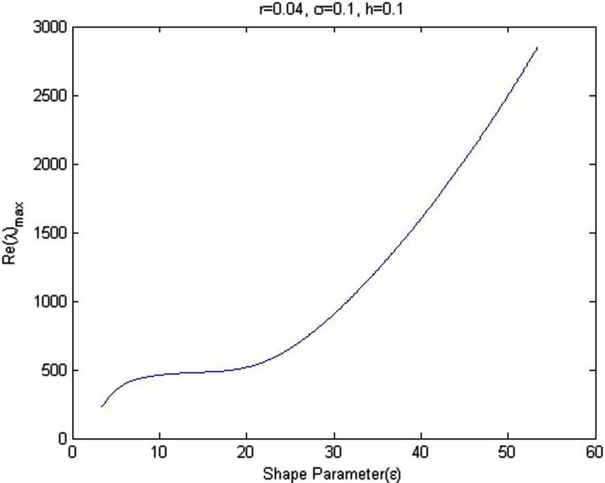
The relation between
and shape parameter
.
Fig. 1 shows maximum eigenvalue
of matrix B varies as a function of shape parameter ε, when mesh spacing parameter h is constant. Fig. 2 shows the effect of mesh length ‘h’ for eigenvalue of matrix B, when the shape parameter
is constant. Fig. 3 shows that the increasing of volatility trends to decreasing of maximum eigenvalue at the end. In this case, if the shape parameter increase then eigenvalue
will increase. Fig. 4 presents that the risk free interest rate is stable for all case of shape parameter and the shape parameter increase then eigenvalue
will increase (see Figs. 5–14).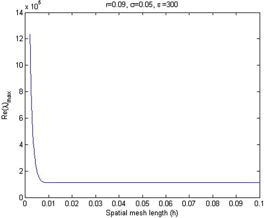
The relation between
and spatial mesh length (h).
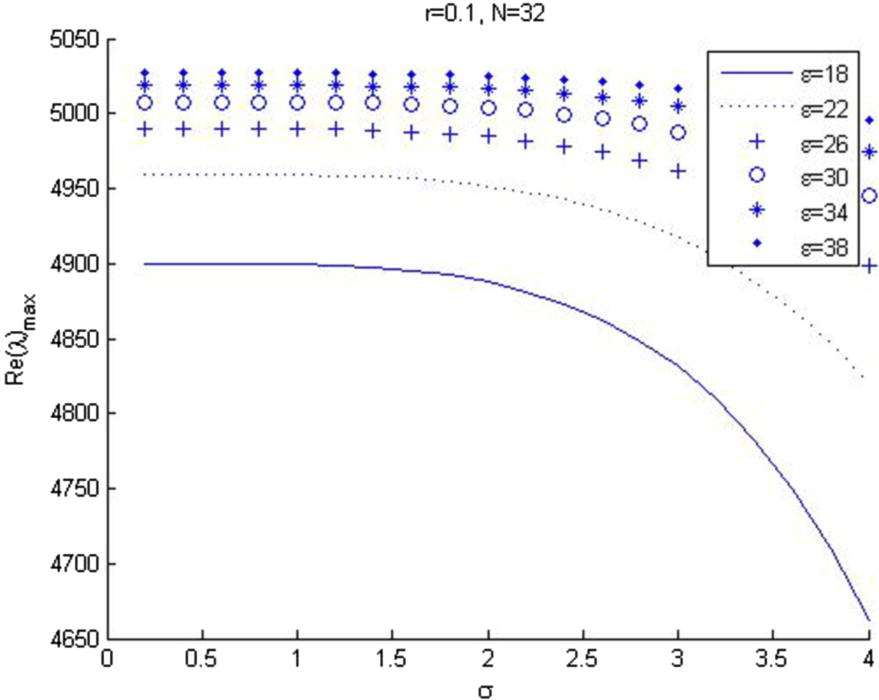
The relation between
and the volatility (σ).
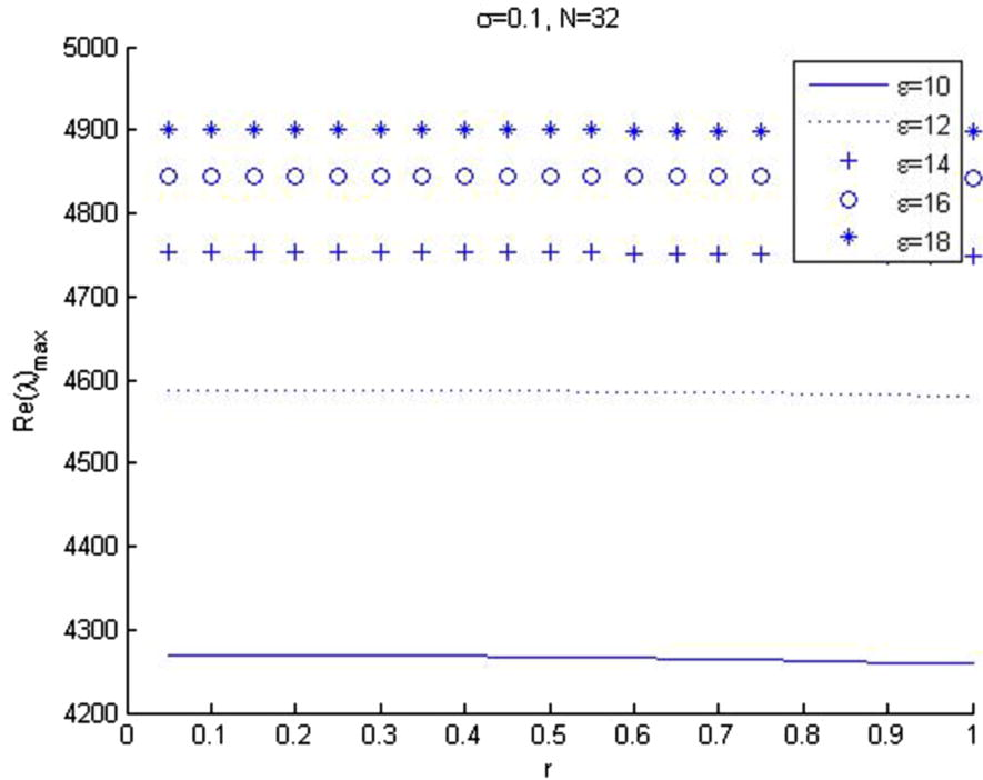
The relation between
and risk free interest rate (r).
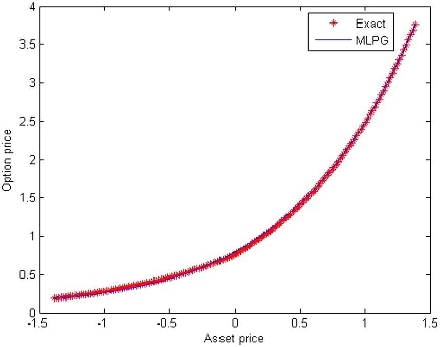
The approximate solution compare with the exact solution for
.
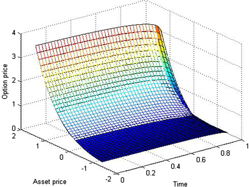
The approximate solution compare with the exact solution for
.
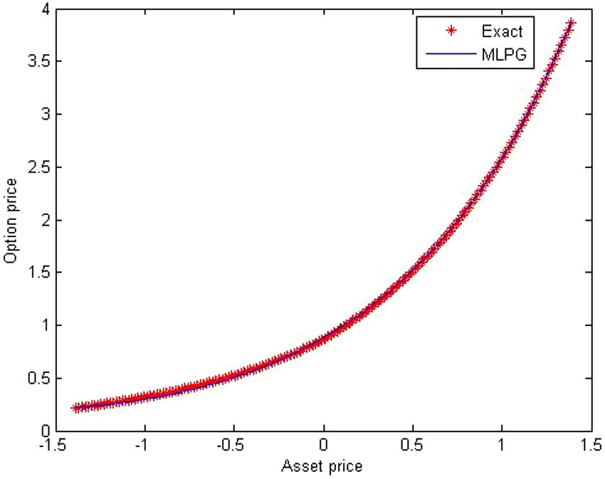
The approximate solution compare with the exact solution for σ = 0.2, r = 0.04, α = 0.99, t = T.
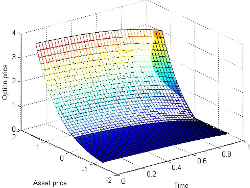
The approximate solution compare with the exact solution for
.
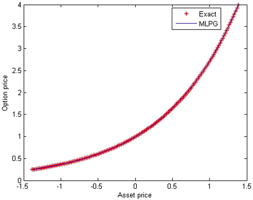
The approximate solution compare with the exact solution for
.
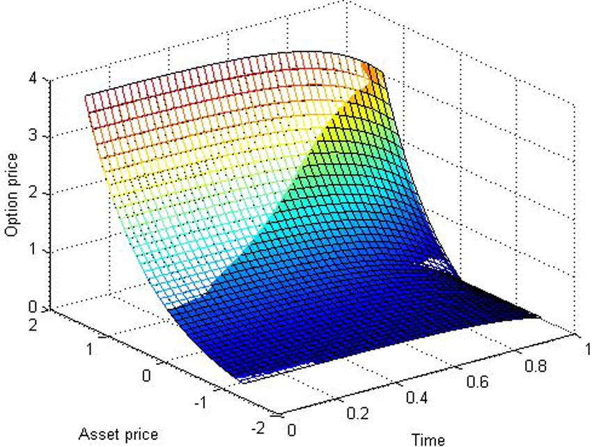
The approximate solution compare with the exact solution for
.
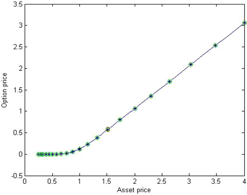
The comparison of the approximate solutions of the fractional and standard Black–Scholes equation for
.
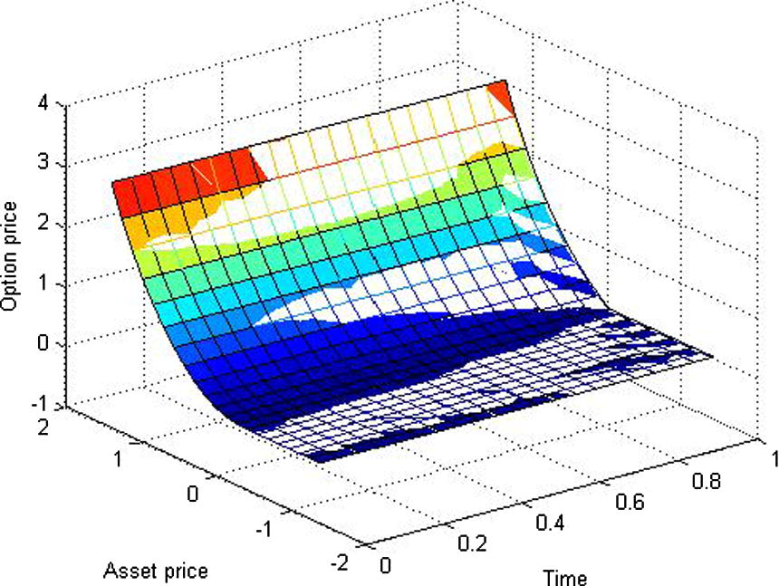
The comparison of the approximate solutions of the fractional and standard Black–Scholes equation for
.
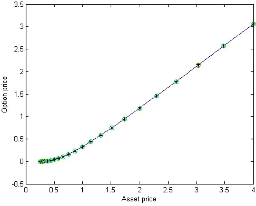
The comparison of the approximate solutions of the fractional and standard Black–Scholes equation for
.
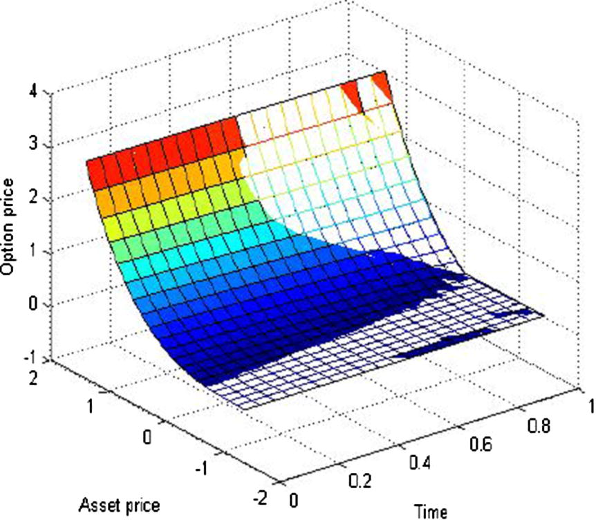
The comparison of the approximate solutions of the fractional and standard Black–Scholes equation for
.
6 Numerical examples
In this section, we are going to present various numerical results to evaluate proposed meshless approaches. Using the MLPG2 method, the resulting problems for European call options are solved via implicit finite difference method.
The European call option can be modeled by Black–Scholes PDE
To illustrate accuracy of proposed method numerical simulation was done for European call option with parameters xmin = −ln (4E), xmax = ln (4E).
6.1 Example 1
We consider the fractional Black–Scholes equation in Eq. (3.1). The numerical simulation was done for European call option with parameters as following:
Case 1. For σ = 0.2, r = 0.04, α = 0.5, T = 1.
Case 3. For σ = 0.2, r = 0.04, α = 0.99, T = 1.
Case 4. For σ = 0.2, r = 0.1, α = 0.99, T = 1.
6.2 Example 2
We consider the fractional Black–Scholes equation in Eq. (5.1). The numerical simulation was done for European call option with parameters as following:
Case 1. For σ = 0.15(0.5 + 2τ)((s/100 − 1.2)2/((s/100)2 + 1.44)), r = 0.06, α = 0.99, T = 1.
xmin = −ln (4E), xmax = ln (4E).
In this case, we have unknown the exact solution.
Case 2. For σ = 0.4(2 + sin x), r = 0.06, α = 0.99, T = 1. In this case, we have unknown the exact solution.
7 Conclusion
In this paper, the fractional Black–Scholes equation are solved by the implicit finite difference method and MLPG2 for discretizing in time variable and option price, respectively. The stability analysis present relation between maximum eigenvalues of matrix and variety of parameters.
The numerical results are presented in two examples. Example 1 presents numerical results for varieties of parameters in four cases. For case 1 and case 2 present comparison of numerical result for different volatility σ = 0.1, 0.2 while variables are fixed, α = 0.5, 0.99 show for case 2 and case 3. Difference of risk free interest rate present for case 3 and case 4, respectively. Example 2 shows the value of option for volatility function in both cases. Volatility function is σ = 0.15(0.5 + 2τ)((s/100 − 1.2)2/((s/100)2 + 1.44)) and σ = 0.4(2 + sin x), respectively. Moreover, we found that the MLPG give the value option in both volatility constant and volatility function.
Acknowledgements
This research is partially supported by King Mongkut’s University of Technology Thonburi (KMUTT). The authors would like to thank their advisor for providing advice and taking care of this research and Rajamangala University of Technology Krungthep for providing a scholarship.
References
- Analysis of Keller–Segel model with a fractional derivative without singular kernel. Entropy. 2015;17:4439-4453.
- [Google Scholar]
- Extension of resistance, inductance, capacitance electrical circuit to fractional derivative without singular kernel. Adv. Mech. Eng.. 2015;7:1-6.
- [Google Scholar]
- The meshless local Petrov–Galerkin (MLPG) method: a simple & less-costly alternative to the finite element and boundary element methods. CMES. 2002;3(1):11-51.
- [Google Scholar]
- Option pricing with transaction costs and a nonlinear Black–Scholes equation. Finance Stochast.. 1998;2:369-397.
- [Google Scholar]
- A note on wick products and the fractional Black–Scholes model. Finance Stochast.. 2005;9:197-209.
- [Google Scholar]
- The pricing of options and corporate liabilities. J. Political Econ.. 1973;81(3):637-654.
- [Google Scholar]
- Elasticita e Dissipazione. Bologna: Zani-Chelli; 1969.
- European option pricing with transaction costs. SIAM J. Control Optim. 1993:470-493.
- [Google Scholar]
- European option pricing of fractional Black–Scholes model with new Lagrange multipliers. Comput. Methods Differ. Equ.. 2014;2(1):1-10.
- [Google Scholar]
- Cubic spline method for a generalized Black–Scholes equation. Math. Prob. Eng.. 2014;7(3):229-235.
- [Google Scholar]
- The pricing of options on asset with stochastic volatilities. J. Finance. 1987;42:281-300.
- [Google Scholar]
- Ishteva, M.K., 2005. Properties and applications of the Caputo fractional operator (Master thesis). Karlsruhe Univ, Sofia.
- Option when underlying stock returns are discontinuous. J. Financial Econ.. 1976;3:125-144.
- [Google Scholar]
- Implicit finite difference approximation for time fractional diffusion equations. Comput. Math. Appl.. 2008;56:1138-1145.
- [Google Scholar]
- Fractional Differential Calculus. New York: Academic Press; 1999.
- Solution of the fractional Black–Scholes option pricing model by finite difference method. Abstr. Appl. Anal.. 2013;2013:194286 10 pages
- [CrossRef] [Google Scholar]
- Scaling and long-range dependence in option pricing I: pricing European option with transaction costs under the fractional Black–Scholes model. Physica 2010:438-444.
- [Google Scholar]


