The Marshall–Olkin–Weibull-H family: Estimation, simulations, and applications to COVID-19 data

Ahmed Z. Afify; Hazem Al-Mofleh; Hassan M. Aljohani; Gauss M. Cordeiro

doi:10.1016/j.jksus.2022.102115

View/Download PDF

Buy Reprints

PDF

Translate this page into:

Original article

07 2022

:34;

102115

doi:

10.1016/j.jksus.2022.102115

The Marshall–Olkin–Weibull-H family: Estimation, simulations, and applications to COVID-19 data

Ahmed Z. Afify^{^a,⁎}, Hazem Al-Mofleh^{^b}, Hassan M. Aljohani^{^c}, Gauss M. Cordeiro^{^d}

a Department of Statistics, Mathematics and Insurance, Benha University, Benha 13511, Egypt

b Department of Mathematics, Tafila Technical University, Tafila 66110, Jordan

c Department of Mathematics & Statistics, College of Science, Taif University, P.O. Box 11099, Taif 21944, Saudi Arabia

d Department of Statistics, Federal University of Pernambuco, Recife 50710-165, Brazil

⁎Corresponding author.

Received: 2021-12-3, Accepted: 2022-5-17,

Disclaimer:
This article was originally published by Elsevier and was migrated to Scientific Scholar after the change of Publisher.

Abstract

We define a new extended Weibull-H family and obtain some of its mathematical properties. It is very competitive to the beta-G and Kumaraswamy-G classes, which are highly cited in Google Scholar. The parameters of a specified sub-model are estimated by eight methods and its flexibility is proved in two applications to COVID-19 data.

Keywords

COVID-19 data

Generalized distribution

Maximum likelihood estimation

Weibull distribution

1 Introduction

Adding one or two parameters to parent distributions encourage new concepts for flexible modeling in distribution theory. Among well-established classes of distributions, the exponentiated-G, transmuted-G and Marshall–Olkin-G (MO-G) (Marshall and Olkin, 1997) offer induction of one extra parameter, while the beta-G (Eugene et al., 2002) and Kumaraswamy-G (Cordeiro and de Castro, 2011) classes require two additional shape parameters. Their special cases are explored by Tahir and Nadarajah (2015), among those of other classes.

Composition of distribution generators is emerging as a method to obtain flexible distributions to fit real data in the last five years or so. Some new classes were derived following this method such as the Weibull Marshall–Olkin (Korkmaz et al., 2019), Marshall–Olkin transmuted (Afify et al., 2020), Marshall–Olkin Burr-III (Afify et al., 2021b), among others.

Some other important G families are the exponentiated-G by Gupta et al. (1998), transmuted-G by Shaw and Buckley (2007), gamma-G by Zografos and Balakrishnan (2009), McDonald-G by Alexander et al. (2012), exponentiated-generalized-G by Cordeiro et al. (2013), Burr X-G by Yousof et al. (2017), additive Weibull-G by Hassan and Hemeda (2017), generalized transmuted-G by Nofal et al. (2017), odd Lomax-G by Cordeiro et al. (2019), Kumaraswamy alpha power-G by Mead et al. (2020), modified Kies-G by Al-Babtain et al. (2020), log–logistic tan-G by Zaidi et al. (2021), and generalized linear failure rate-G by Afify et al. (2022). The interested reader can explore more about parameter induction in Tahir and Nadarajah (2015).

Let $H (x; ξ)$ be a baseline cumulative distribution function (CDF) with a parameter vector $ξ$ . Bourguignon et al. (2014) defined the CDF of the Weibull-H (W-H) class with an extra shape parameter $β > 0$ by

(1)

G (x) = G (x; β, ξ) = 1 - \exp \{- {[\frac{H (x)}{\overline{H} (x)}]}^{β}\}, x \in R,

where

\overline{H} (x) = 1 - H (x)

The CDF of the MO-G class is defined by

(2)

F (x) = F (x; Ω) = \frac{G (x)}{θ + (1 - θ) G (x)}, x \in R,

where

θ > 0, G (x)

is a parent CDF, and

Ω = {(θ, ξ^{⊤})}^{⊤}

By combining (1) and (2) (and omitting arguments), the CDF of the Marshall–Olkin–Weibull-H (MOW-H) family (with extra parameters $β$ and $θ$ ) follows as

(3)

F (x) = F (x; Θ) = \frac{1 - \exp \{- {[\frac{H (x)}{\overline{H} (x)}]}^{β}\}}{1 - (1 - θ) \exp \{- {[\frac{H (x)}{\overline{H} (x)}]}^{β}\}}, x \in R,

where

Θ = {(β, θ, ξ^{⊤})}^{⊤}

By differentiating (3), the probability density function (PDF) of the MOW-H family reduces to

(4)

f (x) = f (x; Θ) = \frac{θ β h (x) H {(x)}^{β - 1} \exp \{- {[\frac{H (x)}{\overline{H} (x)}]}^{β}\}}{\overline{H} {(x)}^{β + 1} {\{1 - (1 - θ) \exp \{- {[\frac{H (x)}{\overline{H} (x)}]}^{β}\}\}}^{2}},

where

h (x) = h (x; ξ) = dH (x) / dx

Henceforth, $X \sim MOW - H (β, θ, ξ)$ denotes a random variable (rv) having density (4).

The hazard rate function (HRF) of X is

(5)

HRF (x) = HRF (x; Θ) = \frac{β h (x) H {(x)}^{β - 1} \overline{H} {(x)}^{- β - 1}}{1 - (1 - θ) \exp \{- {[\frac{H (x)}{\overline{H} (x)}]}^{β}\}} .

By inverting $F (x) = u$ in Eq. (3), we can obtain the quantile function (QF) of X as $x = Q_{X} (u) = H^{- 1} (v / [1 + v])$ , where $v = v (u) = {[- \log (t)]}^{1 / β}$ and $t = t (u) = (1 - u) / [1 - (1 - θ) u]$ .

A simple interpretation of the MOW-H family can be given as follows. Consider that the variability of the odds $H (x) / \overline{H} (x)$ of a rv Z follows a Weibull distribution with unity scale and shape $β$ . Let N be a positive integer rv having a geometric distribution with parameter $δ$ , say $P (N = n) = δ {(1 - δ)}^{n - 1}$ (for $n = 1, 2, \dots$ ). Consider a sequence of N independent copies of Z obtained independently of N. Setting the probability parameters $δ = θ$ and $δ = 1 / θ$ for $θ \in (0, 1)$ and $θ > 1$ , respectively, the minimum of $Z_{1}, \dots, Z_{n}$ has PDF (4).

Furthermore, the proposed MOW-H family extends the Weibull-G class (Bourguignon et al., 2014) which has 536 citations so far, and then it is more flexible than the Weibull-G class. In fact, the plots in Figs. 1 to 8 reveal that the two extra parameters to the baseline model makes the density and risk functions of the new family much more flexible for the four baseline distributions considered here. Additionally, the proposed family can be a competitive generator to the beta-G (Eugene et al., 2002) and Kumaraswamy-G (Cordeiro and de Castro, 2011) classes, which also require two additional shape parameters. These two classes are among the most cited papers in the distribution theory literature.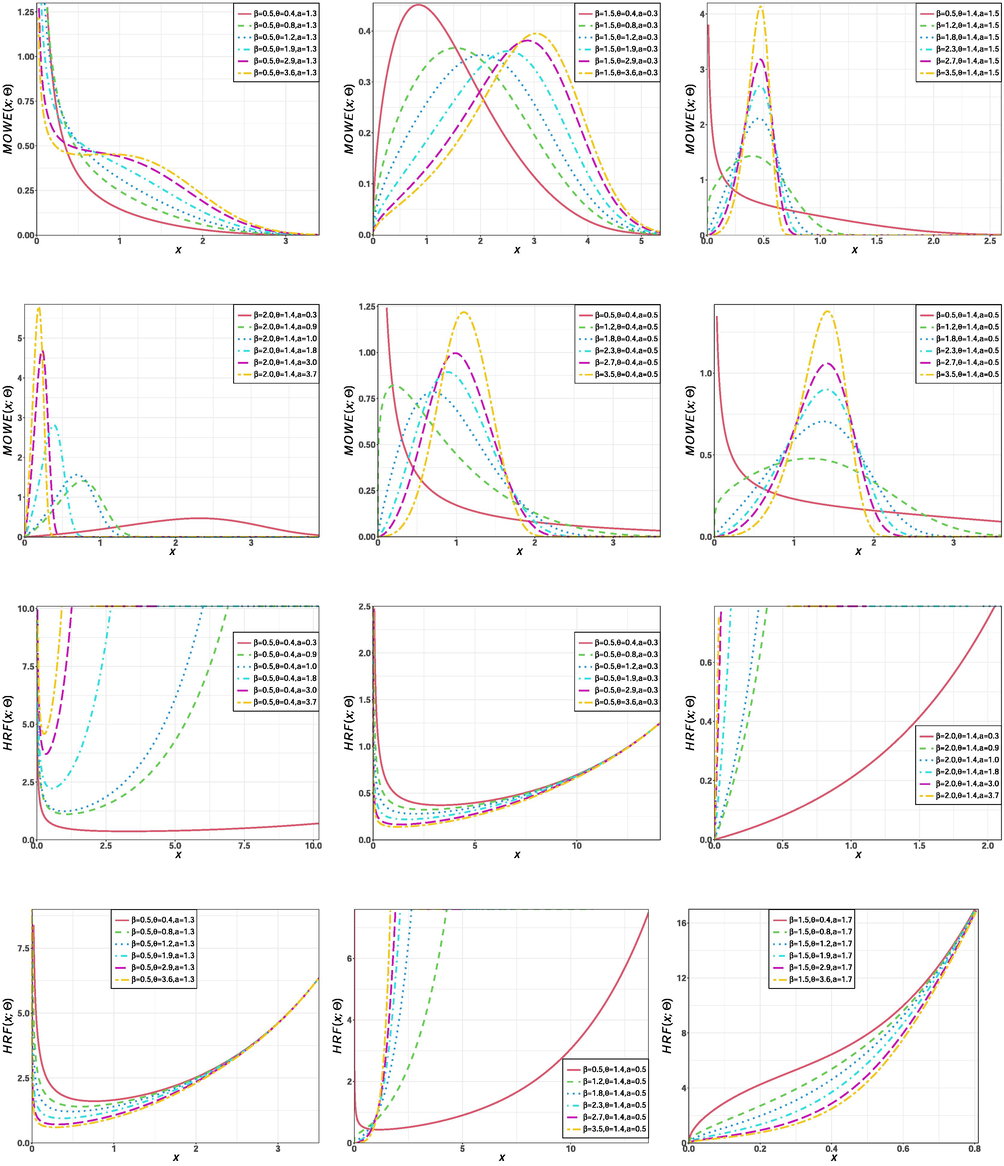

Shapes of density and hazard functions of the MOWE model for different parameter values.

The paper is structured as follows: Section 2 provides four special cases of Eq. (4), and Section 3 addresses some properties of the new family. Section 4 provides the parameter estimation by eight methods. Two applications to COVID-19 data in Section 6 illustrate the utility of the new family. Section 6 ends with some conclusions.

2 Special Models

This section is devoted to introducing some special sub-models of the MOW-H family. The two extra shape parameters of the MOW-H family make the baseline hazard function more flexible to exhibit all important hazard rate shapes, including monotone and non-monotone shapes.

2.1

2.1 MOW-exponential (MOWE)

The MOWE density follows from the exponential Exp $(a)$ distribution, where $a > 0$ . The PDF and CDF of the MOWE distribution are (for $x \in R$ ), respectively,

(6)

f_{MOWE} (x) = \frac{θ β a {[\exp (- a x)]}^{- β} {[1 - \exp (- a x)]}^{β - 1} \exp \{- {[\exp (a x) - 1]}^{β}\}}{{\{θ + (1 - θ) [1 - \exp \{- {[\exp (a x) - 1]}^{β}\}]\}}^{2}}

and

(7)

F_{MOWE} (x) = \frac{1 - \exp \{- {[\exp (a x) - 1]}^{β}\}}{1 - (1 - θ) \exp \{- {[\exp (a x) - 1]}^{β}\}} .

The QF of the MOWE model (for

0 < u < 1

) reduces to

(8)

Q_{MOWE} (u) = - \frac{1}{a} \log \{1 - \frac{{(- \log [\frac{u - 1}{u (1 - θ) - 1}])}^{1 / β}}{{(- \log [\frac{u - 1}{u (1 - θ) - 1}])}^{1 / β} + 1}\} .

Fig. 1 displays shapes of the PDF and HRF for some parameters. The HRF can assume increasing, decreasing, reversed-J and J shapes.

2.2

2.2 MOW-uniform (MOWU)

For the uniform in the interval $(0, α), H (x) = x / α$ , where $α > 0$ . Then, the PDF of the MOWU model has the form (for $x \in (0, α)$ ) $f_{MOWU} (x) = \frac{θ β α^{- 1} {(x / α)}^{β - 1} \exp \{- {[x / (α - x)]}^{β}\}}{{(1 - x / α)}^{β + 1} {\{θ + (1 - θ) [1 - \exp \{- {(x / α)}^{β}\}]\}}^{2}} .$

The Weibull-uniform density when $θ = 1$ was derived by Phani (1987).

2.3

2.3 MOW-Lomax (MOWL)

The Lomax distribution has CDF $H (x) = 1 - {(1 + x / λ)}^{- α}$ (for $x ⩾ 0$ ), where $α > 0$ is a shape, and $λ > 0$ is a scale. The PDF of the MOWL model (for $x \in R$ ) is $f_{MOWL} (x) = \frac{θ β α {[1 - {(1 + x / λ)}^{- α}]}^{β - 1} \exp \{- {[{(1 + x / λ)}^{α} - 1]}^{β}\}}{λ {(1 + x / λ)}^{1 - α β} {\{θ + (1 - θ) [1 - \exp \{- {[{(1 + x / λ)}^{α} - 1]}^{β}\}]\}}^{2}} .$

2.4

2.4 MOW-Weibull (MOWW)

The CDF of the Weibull is $H (x) = 1 - \exp {- λ x^{γ}}$ , where $λ > 0$ and $γ > 0$ , and the MOWW density (for $x \in R$ ) has the form

(9)

f_{MOWW} (x) = \frac{θ β λ γ x^{γ - 1} \exp (- λ x^{γ}) {[1 - \exp (- λ x^{γ})]}^{β - 1} \exp \{- {[\exp (λ x^{γ}) - 1]}^{β}\}}{\exp [- λ (β + 1) x^{γ}] {\{θ + (1 - θ) [1 - \exp \{- {[\exp (λ x^{γ}) - 1]}^{β}\}]\}}^{2}} .

The MOWW model includes the exponential power (Smith and Bain, 1975) and the Chen (2000) distribution when $θ = β = 1$ and $θ = β = λ = 1$ , respectively.

3 Properties

The PDF associated with the CDF (2) admits the linear representation (Cordeiro et al., 2014)

(10)

f (x) = \sum_{k = 0}^{\infty} w_{k} π_{k + 1} (x),

where

π_{k + 1} (x) = (k + 1) g (x) G {(x)}^{k}

is the exponentiated-G (“exp-G”) density with power parameter

k + 1

w_{k} = [p_{k} I_{(0, 1)} (θ) + q_{k} I_{(1, \infty)} (θ)],

$I_{A} (z)$ is the indicator function of a subset A, $p_{k} = \frac{{(- 1)}^{k} θ}{(k + 1)} \sum_{j = k}^{\infty} (j + 1) (\begin{matrix} j \\ k \end{matrix}) {\bar{θ}}^{j}$ and $q_{k} = θ^{- 1} {(1 - θ^{- 1})}^{k}$ .

By inserting Eq. (1) and its derivative in $π_{k + 1} (x)$ and using the expansions for the binomial and exponential function, we obtain (for $k ⩾ 0$ )

(11)

f (x) = \sum_{r, m = 0}^{\infty} q_{r, m} ρ_{(r + 1) β + m} (x),

where

δ_{r}^{(k)} = \sum_{j = 0}^{k} {(- 1)}^{j + r} {(j + 1)}^{r} (\begin{matrix} k \\ j \end{matrix})

q_{r, m} = β \sum_{k = 0}^{\infty} \frac{{(- 1)}^{m} (k + 1) (\begin{matrix} - (r + 1) β - 1 \\ m \end{matrix}) δ_{r}^{(k)}}{(r + 1) β + m} w_{k},

and

ρ_{(r + 1) β + m} (x)

is the exp-H density with power

(r + 1) β + m

So, the density of X is a double linear combination of exp-H densities, which can be adopted with most common type of software, MAPLE, Mathematica, Ox and R, among others.

3.1

3.1 Moments

Henceforth, $Z_{(r + 1) β + m}$ denotes a rv with PDF $ρ_{(r + 1) β + m} (x)$ . Eq. (11) gives

(12)

μ_{n}^{'} = E (X^{n}) = \sum_{r, m = 0}^{\infty} q_{r, m} E [Z_{(r + 1) β + m}^{n}] = \sum_{r, m = 0}^{\infty} [(r + 1) β + m] q_{r, m} s_{r, m}^{(n)},

where

s_{r, m}^{(n)} = \int_{- \infty}^{\infty} x^{n} h (x) H {(x)}^{(r + 1) β + m - 1} dt = \int_{0}^{1} Q_{H} {(u)}^{n} u^{(r + 1) β + m - 1} du

can be calculated at least numerically from the exp-H moments or via the baseline QF.

Expressions for several exp-H moments (under special baselines) are reported in many papers such as Nadarajah and Kotz (2006).

The nth incomplete moment of X, say $m_{n} (y) = E (X | X ⩽ y)$ , follows as

(13)

m_{n} (y) = \int_{- \infty}^{y} x^{n} f (x) dx = \sum_{r, m = 0}^{\infty} [(r + 1) β + m] q_{r, m} t_{r, m}^{(n)} (y),

where

t_{r, m}^{(n)} (y) = \int_{- \infty}^{y} x^{n} h (x) H {(x)}^{(r + 1) β + m - 1} dt = \int_{0}^{Q_{H} (y)} Q_{H} {(u)}^{n} u^{(r + 1) β + m - 1} du .

The mean deviations and Bonferroni and Lorenz curves of X can be determined from (13) with $n = 1$ .

3.2

3.2 Generating function

The generating function (gf) of X follows from (11) as $M (s) = \sum_{r, m = 0}^{\infty} q_{r, m} M_{(r + 1) β + m} (s) = \sum_{r, m = 0}^{\infty} [(r + 1) β + m] [(r + 1) β + m] q_{r, m} v_{r, m} (s),$ where $M_{(r + 1) β + m} (s)$ is the gf of the exp-H density $ρ_{(r + 1) β + m} (x)$ $v_{r, m} (s) = \int_{- \infty}^{\infty} e^{sx} h (x) H {(x)}^{(r + 1) β + m} dx = \int_{0}^{1} \exp \{s Q_{H} (u)\} u^{(r + 1) β + m} du .$

4 Estimation in the MOWE model

Let $x_{1}, \dots, x_{n}$ be observations from the MOWE distribution (Section 2.2), and $x_{(1)}, \dots, x_{(n)}$ be the order statistics. The CDF and PDF of this model are denoted by $F (\cdot)$ and $f (\cdot)$ , respectively. Its parameters can be estimated by eight methods described below. For more information about these estimation methods, see Nassar et al. (2018), Ramos et al. (2018), Rodrigues et al. (2018), and Ramos et al. (2019).

The ordinary least-squares estimates (OLSEs) minimize the function $V (β, θ, a) = \sum_{i = 1}^{n} {[F (x_{i}) - \frac{i}{n + 1}]}^{2} .$

They can also be found by solving the non-linear equations $\sum_{i = 1}^{n} [F (x_{i}) - \frac{i}{n + 1}] Δ_{s} (x_{i}) = 0, s = 1, 2, 3,$ where $Δ_{1} (x_{i}) = Δ_{1} (x_{i} | β, θ, a)$ , $Δ_{2} (x_{i}) = Δ_{2} (x_{i} | β, θ, a)$ and $Δ_{3} (x_{i}) = Δ_{3} (x_{i} | β, θ, a)$ are $Δ_{1} (x_{i}) = \frac{\partial F (x_{i})}{\partial β} = θ \frac{{(e^{{ax}_{i}} - 1)}^{β} e^{- {(e^{{ax}_{i}} - 1)}^{β}} \log (e^{{ax}_{i}} - 1)}{{[1 - (1 - θ) e^{- {(e^{{ax}_{i}} - 1)}^{β}}]}^{2}},$ $Δ_{2} (x_{i}) = \frac{\partial F (x_{i})}{\partial θ} = - \frac{e^{- {(e^{{ax}_{i}} - 1)}^{β}} [1 - e^{- {(e^{{ax}_{i}} - 1)}^{β}}]}{{[1 - (1 - θ) e^{- {(e^{{ax}_{i}} - 1)}^{β}}]}^{2}}$ and $Δ_{3} (x_{i}) = \frac{\partial F (x_{i})}{\partial a} = \frac{β θ x_{i} [{(e^{{ax}_{i}} - 1)}^{β - 1} e^{{ax}_{i} - {(e^{{ax}_{i}} - 1)}^{β}}]}{{[1 - (1 - θ) e^{- {(e^{{ax}_{i}} - 1)}^{β}}]}^{2}} .$

The weighted least-squares estimates (WLSEs) minimize $W (β, θ, a) = \sum_{i = 1}^{n} \frac{{(n + 1)}^{2} (n + 2)}{i (n - i + 1)} {[F (x_{i}) - \frac{i}{n + 1}]}^{2},$ which follow by solving $\sum_{i = 1}^{n} \frac{{(n + 1)}^{2} (n + 2)}{i (n - i + 1)} [F (x_{i}) - \frac{i}{n + 1}] Δ_{s} (x_{i}) = 0, s = 1, 2, 3 .$

The maximum likelihood estimates (MLEs) maximize the log-likelihood below for the parameters follows from (6) by classical iterative methods

(14)

\begin{matrix} ℓ (Θ) = & \sum_{i = 1}^{n} \log (β θ x_{i}^{β - 1} + θ) - \sum_{i = 1}^{n} (θ x_{i}^{β} + θ x_{i}) \\ + \sum_{i = 1}^{n} \log (1 + e^{- θ x_{i}^{β} - θ x_{i}}) - \sum_{i = 1}^{n} (1 - e^{- θ x_{i}^{β} - θ x_{i}}) . \end{matrix}

The maximum product of spacing estimates (MPSEs) are good alternatives to the MLEs. Let $D_{i} = D_{i} (β, θ, a) = F (x_{(i)}) - F (x_{(i - 1)})$ be the uniform spacing (for $i = 1, \dots, n + 1$ ), where $F (x_{(0)}) = 0, F (x_{(n + 1)}) = 1$ and $\sum_{i = 1}^{n + 1} D_{i} = 1$ . The MPSEs maximize the quantity $H (β, θ, a) = \sum_{i = 1}^{n + 1} \log [D_{i}],$ which can be determined from the non-linear equations $\sum_{i = 1}^{n + 1} \frac{1}{D_{i}} [Δ_{s} (x_{(i)}) - Δ_{s} (x_{(i - 1})] = 0, s = 1, 2, 3 .$

The Cramér-von Mises estimates (CVMEs) minimize $C (β, θ, a) = - \frac{1}{12 n} + \sum_{i = 1}^{n} {[F (x_{i}) - \frac{2 i - 1}{2 n}]}^{2},$ which also follow by solving $\sum_{i = 1}^{n} [F (x_{i}) - \frac{2 i - 1}{2 n}] Δ_{s} (x_{i}) = 0, s = 1, 2, 3 .$

The Anderson–Darling estimates (ADEs) minimize $A (β, θ, a) = - n - \frac{1}{n} \sum_{i = 1}^{n} (2 i - 1) [\log F (x_{i}) + \log S (x_{i})],$ which can be found as solutions of the system $\sum_{i = 1}^{n} (2 i - 1) [\frac{Δ_{s} (x_{i})}{F (x_{i})} - \frac{Δ_{i} (x_{n + 1 - i})}{S (x_{n + 1 - i})}] = 0, s = 1, 2, 3 .$

The right-tail Anderson–Darling estimates (RADEs) minimize $R (β, θ, a) = \frac{n}{2} - 2 \sum_{i = 1}^{n} F (x_{(i)}) - \frac{1}{n} \sum_{i = 1}^{n} (2 i - 1) \log S (x_{(n + 1 - i)}) .$

They can also be obtained from the non-linear equations $- 2 \sum_{i = 1}^{n} Δ_{s} (x_{(i)}) + \frac{1}{n} \sum_{i = 1}^{n} (2 i - 1) \frac{Δ_{s} (x_{(n + 1 - i)})}{S (x_{(n + 1 - i)})} = 0, s = 1, 2, 3 .$

Let $u_{i} = i / (n + 1)$ be an unbiased estimator of $F (x_{(i})$ . The PC estimates (PCEs) minimize $P (β, φ, ρ) = \sum_{i = 1}^{n} {(x_{(i)} - \frac{1}{β} \log [\sqrt{- \log (1 - {(\frac{1}{2 ρ} [(ρ + 1) - \sqrt{δ (ρ, u_{i})}])}^{1 / ϕ})} + 1])}^{2},$ where $δ (ρ, u_{i}) = {(ρ + 1)}^{2} - 4 ρ u_{i}$ .

5 Simulation analysis

The simulation study compares the estimates from the eight methods in Section 4 in terms of the averages of the four quantities: absolute bias ( $| Bias (\hat{θ}) |$ ), $| Bias (\hat{θ}) | = \frac{1}{N} \sum_{i = 1}^{N} | \hat{θ} - θ |$ , mean square error (MSE), $MSE = \frac{1}{N} \sum_{i = 1}^{N} {(\hat{θ} - θ)}^{2}$ , and mean relative error (MRE), $MRE = \frac{1}{N} \sum_{i = 1}^{N} | \hat{θ} - θ | / θ$ .

The observations from the MOWE model are simulated from Eq. (8), where U is a uniform random variable in the interval $(0, 1)$ . We generate $N = 5, 000$ random samples $x_{1}, \dots, x_{n}$ (for $n = 30, 50, 80, 120$ , and 200) from the MOWE model with $β = {0.2, 1.0, 2.1}, θ = {0.1, 1.1, 1.2}$ and $a = {0.5, 1.5, 4.7}$ .We use R codes (R Core Team, 2020, version 4.0.3) for the simulations and the nlminb function in the stats package (R Core Team, 2020, version 4.0.3).

We estimate its parameters for some parameter combinations and sample sizes, and calculate the MSEs and MREs of the estimates. Four out of twenty-seven simulated outcomes are reported in Tables 1–4 , whose numbers in each row have superscripts giving the ranks of the estimates among all methods, and $\sum Ranks$ denotes the partial sum of the ranks.

Table 1 Simulation results for

β = 0.2, θ = 0.1, a = 0.5

$n$	Est.	Est. Par.	WLSE	OLSE	MLE	MPSE	CVME	ADE	RADE	PCE
30	$\| BIAS \|$	$\hat{β}$	${0.03046}^{{3}}$	${0.03238}^{{4}}$	${0.03296}^{{5}}$	${0.01676}^{{1}}$	${0.03496}^{{6}}$	${0.02049}^{{2}}$	${0.03627}^{{7}}$	${0.13516}^{{8}}$
		$\hat{θ}$	${0.05229}^{{4}}$	${0.05604}^{{6}}$	${0.03758}^{{3}}$	${0.03074}^{{1}}$	${0.05540}^{{5}}$	${0.03340}^{{2}}$	${0.05803}^{{7}}$	${0.09540}^{{8}}$
		$\hat{a}$	${0.25949}^{{5}}$	${0.24201}^{{4}}$	${0.16096}^{{2}}$	${0.11232}^{{1}}$	${0.26435}^{{6}}$	${0.17529}^{{3}}$	${0.42485}^{{7}}$	${0.61630}^{{8}}$
	MSE	$\hat{β}$	${0.00156}^{{3}}$	${0.00171}^{{4}}$	${0.00658}^{{7}}$	${0.00073}^{{1}}$	${0.00215}^{{5}}$	${0.00116}^{{2}}$	${0.00227}^{{6}}$	${0.03304}^{{8}}$
		$\hat{θ}$	${0.00503}^{{3}}$	${0.00597}^{{5}}$	${0.00658}^{{7}}$	${0.00279}^{{1}}$	${0.00574}^{{4}}$	${0.00318}^{{2}}$	${0.00603}^{{6}}$	${0.01496}^{{8}}$
		$\hat{a}$	${0.14750}^{{5}}$	${0.14370}^{{4}}$	${0.10088}^{{2}}$	${0.05369}^{{1}}$	${0.17974}^{{6}}$	${0.10141}^{{3}}$	${0.28668}^{{7}}$	${0.48110}^{{8}}$
	MRE	$\hat{β}$	${0.15231}^{{3}}$	${0.16191}^{{4}}$	${0.16482}^{{5}}$	${0.08382}^{{1}}$	${0.17479}^{{6}}$	${0.10244}^{{2}}$	${0.18136}^{{7}}$	${0.67578}^{{8}}$
		$\hat{θ}$	${0.52285}^{{4}}$	${0.56041}^{{6}}$	${0.37581}^{{3}}$	${0.30738}^{{1}}$	${0.55401}^{{5}}$	${0.33404}^{{2}}$	${0.58032}^{{7}}$	${0.95399}^{{8}}$
		$\hat{a}$	${0.51897}^{{5}}$	${0.48402}^{{4}}$	${0.32192}^{{2}}$	${0.22464}^{{1}}$	${0.52870}^{{6}}$	${0.35058}^{{3}}$	${0.84970}^{{7}}$	${1.23259}^{{8}}$
	$\sum Ranks$		$35^{{3}}$	$41^{{5}}$	$36^{{4}}$	$9^{{1}}$	$49^{{6}}$	$21^{{2}}$	$61^{{7}}$	$72^{{8}}$

50	$\| BIAS \|$	$\hat{β}$	${0.02321}^{{4}}$	${0.02559}^{{5}}$	${0.02135}^{{3}}$	${0.00978}^{{1}}$	${0.02579}^{{6}}$	${0.01157}^{{2}}$	${0.02691}^{{7}}$	${0.13480}^{{8}}$
		$\hat{θ}$	${0.04096}^{{4}}$	${0.04494}^{{7}}$	${0.02332}^{{3}}$	${0.01626}^{{1}}$	${0.04267}^{{5}}$	${0.01885}^{{2}}$	${0.04381}^{{6}}$	${0.07792}^{{8}}$
		$\hat{a}$	${0.22675}^{{5}}$	${0.22534}^{{4}}$	${0.07521}^{{2}}$	${0.04893}^{{1}}$	${0.23677}^{{6}}$	${0.10847}^{{3}}$	${0.34806}^{{7}}$	${0.61778}^{{8}}$
	MSE	$\hat{β}$	${0.00088}^{{3}}$	${0.00106}^{{4}}$	${0.00460}^{{7}}$	${0.00034}^{{1}}$	${0.00111}^{{5}}$	${0.00046}^{{2}}$	${0.00121}^{{6}}$	${0.03037}^{{8}}$
		$\hat{θ}$	${0.00289}^{{3}}$	${0.00369}^{{6}}$	${0.00502}^{{7}}$	${0.00092}^{{1}}$	${0.00317}^{{4}}$	${0.00123}^{{2}}$	${0.00330}^{{5}}$	${0.00934}^{{8}}$
		$\hat{a}$	${0.12574}^{{4}}$	${0.13727}^{{5}}$	${0.03648}^{{2}}$	${0.01628}^{{1}}$	${0.15866}^{{6}}$	${0.05574}^{{3}}$	${0.21190}^{{7}}$	${0.48144}^{{8}}$
	MRE	$\hat{β}$	${0.11607}^{{4}}$	${0.12793}^{{5}}$	${0.10674}^{{3}}$	${0.04888}^{{1}}$	${0.12894}^{{6}}$	${0.05786}^{{2}}$	${0.13456}^{{7}}$	${0.67399}^{{8}}$
		$\hat{θ}$	${0.40965}^{{4}}$	${0.44943}^{{7}}$	${0.23319}^{{3}}$	${0.16259}^{{1}}$	${0.42672}^{{5}}$	${0.18848}^{{2}}$	${0.43811}^{{6}}$	${0.77924}^{{8}}$
		$\hat{a}$	${0.45350}^{{5}}$	${0.45068}^{{4}}$	${0.15041}^{{2}}$	${0.09786}^{{1}}$	${0.47353}^{{6}}$	${0.21694}^{{3}}$	${0.69612}^{{7}}$	${1.23557}^{{8}}$
	$\sum Ranks$		$36^{{4}}$	$47^{{5}}$	$32^{{3}}$	$9^{{1}}$	$49^{{6}}$	$21^{{2}}$	$58^{{7}}$	$72^{{8}}$

80	$\| BIAS \|$	$\hat{β}$	${0.01809}^{{4}}$	${0.01970}^{{5}}$	${0.01470}^{{3}}$	${0.00509}^{{1}}$	${0.02059}^{{6}}$	${0.00615}^{{2}}$	${0.02141}^{{7}}$	${0.13888}^{{8}}$
		$\hat{θ}$	${0.03232}^{{4}}$	${0.03435}^{{5}}$	${0.01345}^{{3}}$	${0.00809}^{{1}}$	${0.03504}^{{7}}$	${0.00991}^{{2}}$	${0.03492}^{{6}}$	${0.06194}^{{8}}$
		$\hat{a}$	${0.20932}^{{5}}$	${0.19572}^{{4}}$	${0.03339}^{{2}}$	${0.01948}^{{1}}$	${0.21641}^{{6}}$	${0.06018}^{{3}}$	${0.26982}^{{7}}$	${0.54785}^{{8}}$
	MSE	$\hat{β}$	${0.00053}^{{3}}$	${0.00062}^{{4}}$	${0.00445}^{{7}}$	${0.00014}^{{1}}$	${0.00069}^{{5}}$	${0.00020}^{{2}}$	${0.00075}^{{6}}$	${0.03267}^{{8}}$
		$\hat{θ}$	${0.00177}^{{3}}$	${0.00203}^{{4.5}}$	${0.00280}^{{7}}$	${0.00034}^{{1}}$	${0.00204}^{{6}}$	${0.00050}^{{2}}$	${0.00203}^{{4.5}}$	${0.00594}^{{8}}$
		$\hat{a}$	${0.11569}^{{4}}$	${0.11685}^{{5}}$	${0.01272}^{{2}}$	${0.00463}^{{1}}$	${0.14005}^{{7}}$	${0.02705}^{{3}}$	${0.13803}^{{6}}$	${0.40737}^{{8}}$
	MRE	$\hat{β}$	${0.09043}^{{4}}$	${0.09852}^{{5}}$	${0.07352}^{{3}}$	${0.02547}^{{1}}$	${0.10295}^{{6}}$	${0.03076}^{{2}}$	${0.10704}^{{7}}$	${0.69439}^{{8}}$
		$\hat{θ}$	${0.32319}^{{4}}$	${0.34354}^{{5}}$	${0.13450}^{{3}}$	${0.08091}^{{1}}$	${0.35035}^{{7}}$	${0.09908}^{{2}}$	${0.34916}^{{6}}$	${0.61944}^{{8}}$
		$\hat{a}$	${0.41865}^{{5}}$	${0.39144}^{{4}}$	${0.06677}^{{2}}$	${0.03895}^{{1}}$	${0.43282}^{{6}}$	${0.12036}^{{3}}$	${0.53963}^{{7}}$	${1.09570}^{{8}}$
	$\sum Ranks$		$36^{{4}}$	${41.5}^{{5}}$	$32^{{3}}$	$9^{{1}}$	$56^{{6}}$	$21^{{2}}$	${56.5}^{{7}}$	$72^{{8}}$

120	$\| BIAS \|$	$\hat{β}$	${0.01461}^{{4}}$	${0.01619}^{{5}}$	${0.00693}^{{3}}$	${0.00216}^{{1}}$	${0.01654}^{{6}}$	${0.00297}^{{2}}$	${0.01736}^{{7}}$	${0.13589}^{{8}}$
		$\hat{θ}$	${0.02608}^{{4}}$	${0.02947}^{{7}}$	${0.00563}^{{3}}$	${0.00324}^{{1}}$	${0.02919}^{{6}}$	${0.00479}^{{2}}$	${0.02868}^{{5}}$	${0.05220}^{{8}}$
		$\hat{a}$	${0.17090}^{{4}}$	${0.18720}^{{5}}$	${0.01370}^{{2}}$	${0.00637}^{{1}}$	${0.19666}^{{6}}$	${0.03035}^{{3}}$	${0.21761}^{{7}}$	${0.47641}^{{8}}$
	MSE	$\hat{β}$	${0.00034}^{{3}}$	${0.00042}^{{4}}$	${0.00223}^{{7}}$	${0.00005}^{{1}}$	${0.00045}^{{5}}$	${0.00008}^{{2}}$	${0.00048}^{{6}}$	${0.03406}^{{8}}$
		$\hat{θ}$	${0.00113}^{{4}}$	${0.00149}^{{7}}$	${0.00088}^{{3}}$	${0.00011}^{{1}}$	${0.00141}^{{6}}$	${0.00019}^{{2}}$	${0.00132}^{{5}}$	${0.00417}^{{8}}$
		$\hat{a}$	${0.08650}^{{4}}$	${0.10942}^{{6}}$	${0.00442}^{{2}}$	${0.00091}^{{1}}$	${0.12331}^{{7}}$	${0.01181}^{{3}}$	${0.09265}^{{5}}$	${0.33211}^{{8}}$
	MRE	$\hat{β}$	${0.07304}^{{4}}$	${0.08094}^{{5}}$	${0.03465}^{{3}}$	${0.01080}^{{1}}$	${0.08271}^{{6}}$	${0.01487}^{{2}}$	${0.08681}^{{7}}$	${0.67947}^{{8}}$
		$\hat{θ}$	${0.26083}^{{4}}$	${0.29466}^{{7}}$	${0.05631}^{{3}}$	${0.03235}^{{1}}$	${0.29191}^{{6}}$	${0.04786}^{{2}}$	${0.28683}^{{5}}$	${0.52202}^{{8}}$
		$\hat{a}$	${0.34180}^{{4}}$	${0.37440}^{{5}}$	${0.02740}^{{2}}$	${0.01273}^{{1}}$	${0.39332}^{{6}}$	${0.06069}^{{3}}$	${0.43522}^{{7}}$	${0.95282}^{{8}}$
	$\sum Ranks$		$35^{{4}}$	$51^{{5}}$	$28^{{3}}$	$9^{{1}}$	$54^{{6.5}}$	$21^{{2}}$	$54^{{6.5}}$	$72^{{8}}$

200	$\| BIAS \|$	$\hat{β}$	${0.01152}^{{4}}$	${0.01277}^{{6}}$	${0.00220}^{{3}}$	${0.00045}^{{1}}$	${0.01256}^{{5}}$	${0.00074}^{{2}}$	${0.01306}^{{7}}$	${0.12438}^{{8}}$
		$\hat{θ}$	${0.02074}^{{4}}$	${0.02385}^{{7}}$	${0.00174}^{{3}}$	${0.00065}^{{1}}$	${0.02336}^{{6}}$	${0.00117}^{{2}}$	${0.02155}^{{5}}$	${0.04304}^{{8}}$
		$\hat{a}$	${0.13754}^{{4}}$	${0.17145}^{{6}}$	${0.00326}^{{2}}$	${0.00156}^{{1}}$	${0.18696}^{{7}}$	${0.00731}^{{3}}$	${0.15700}^{{5}}$	${0.39447}^{{8}}$
	MSE	$\hat{β}$	${0.00021}^{{3}}$	${0.00026}^{{4.5}}$	${0.00083}^{{7}}$	${0.00001}^{{1}}$	${0.00026}^{{4.5}}$	${0.00002}^{{2}}$	${0.00027}^{{6}}$	${0.03047}^{{8}}$
		$\hat{θ}$	${0.00070}^{{4}}$	${0.00095}^{{7}}$	${0.00045}^{{3}}$	${0.00001}^{{1}}$	${0.00092}^{{6}}$	${0.00004}^{{2}}$	${0.00075}^{{5}}$	${0.00279}^{{8}}$
		$\hat{a}$	${0.05948}^{{5}}$	${0.09662}^{{6}}$	${0.00107}^{{2}}$	${0.00012}^{{1}}$	${0.11430}^{{7}}$	${0.00225}^{{3}}$	${0.04729}^{{4}}$	${0.24448}^{{8}}$
	MRE	$\hat{β}$	${0.05760}^{{4}}$	${0.06386}^{{6}}$	${0.01099}^{{3}}$	${0.00224}^{{1}}$	${0.06278}^{{5}}$	${0.00372}^{{2}}$	${0.06531}^{{7}}$	${0.62192}^{{8}}$
		$\hat{θ}$	${0.20742}^{{4}}$	${0.23853}^{{7}}$	${0.01741}^{{3}}$	${0.00655}^{{1}}$	${0.23359}^{{6}}$	${0.01174}^{{2}}$	${0.21547}^{{5}}$	${0.43040}^{{8}}$
		$\hat{a}$	${0.27509}^{{4}}$	${0.34290}^{{6}}$	${0.00651}^{{2}}$	${0.00312}^{{1}}$	${0.37392}^{{7}}$	${0.01462}^{{3}}$	${0.31400}^{{5}}$	${0.78894}^{{8}}$
	$\sum Ranks$		$36^{{4}}$	${55.5}^{{7}}$	$28^{{3}}$	$9^{{1}}$	${53.5}^{{6}}$	$21^{{2}}$	$49^{{5}}$	$72^{{8}}$

Table 2 Simulation results for

β = 1.0, θ = 0.1, a = 0.5

$n$	Est.	Est. Par.	WLSE	OLSE	MLE	MPSE	CVME	ADE	RADE	PCE
30	$\| BIAS \|$	$\hat{β}$	${0.18821}^{{4}}$	${0.19683}^{{5}}$	${0.16502}^{{1}}$	${0.17886}^{{2}}$	${0.20095}^{{6}}$	${0.17967}^{{3}}$	${0.20987}^{{7}}$	${0.28430}^{{8}}$
		$\hat{θ}$	${0.14864}^{{5}}$	${0.16855}^{{7}}$	${0.12346}^{{1}}$	${0.13625}^{{3}}$	${0.16485}^{{6}}$	${0.12721}^{{2}}$	${0.13666}^{{4}}$	${0.21117}^{{8}}$
		$\hat{a}$	${0.38120}^{{5}}$	${0.42480}^{{7}}$	${0.28647}^{{1}}$	${0.30892}^{{2}}$	${0.43726}^{{8}}$	${0.32772}^{{4}}$	${0.32536}^{{3}}$	${0.42004}^{{6}}$
	MSE	$\hat{β}$	${0.05515}^{{4}}$	${0.06053}^{{5}}$	${0.04360}^{{1}}$	${0.04795}^{{2}}$	${0.06523}^{{6}}$	${0.05185}^{{3}}$	${0.07054}^{{7}}$	${0.11469}^{{8}}$
		$\hat{θ}$	${0.05069}^{{5}}$	${0.06359}^{{7}}$	${0.03664}^{{1}}$	${0.04405}^{{3}}$	${0.05997}^{{6}}$	${0.03776}^{{2}}$	${0.04610}^{{4}}$	${0.09969}^{{8}}$
		$\hat{a}$	${0.21907}^{{5}}$	${0.25823}^{{6}}$	${0.15469}^{{1}}$	${0.15513}^{{2}}$	${0.27463}^{{8}}$	${0.17103}^{{4}}$	${0.17084}^{{3}}$	${0.26387}^{{7}}$
	MRE	$\hat{β}$	${0.18821}^{{4}}$	${0.19683}^{{5}}$	${0.16502}^{{1}}$	${0.17886}^{{2}}$	${0.20095}^{{6}}$	${0.17967}^{{3}}$	${0.20987}^{{7}}$	${0.28430}^{{8}}$
		$\hat{θ}$	${1.48640}^{{5}}$	${1.68551}^{{7}}$	${1.23455}^{{1}}$	${1.36251}^{{3}}$	${1.64850}^{{6}}$	${1.27207}^{{2}}$	${1.36664}^{{4}}$	${2.11173}^{{8}}$
		$\hat{a}$	${0.76240}^{{5}}$	${0.84960}^{{7}}$	${0.57293}^{{1}}$	${0.61784}^{{2}}$	${0.87451}^{{8}}$	${0.65544}^{{4}}$	${0.65072}^{{3}}$	${0.84008}^{{6}}$
	$\sum Ranks$		$42^{{4.5}}$	$56^{{6}}$	$9^{{1}}$	$21^{{2}}$	$60^{{7}}$	$27^{{3}}$	$42^{{4.5}}$	$67^{{8}}$

50	$\| BIAS \|$	$\hat{β}$	${0.14676}^{{4}}$	${0.15674}^{{5}}$	${0.13258}^{{1}}$	${0.13664}^{{2}}$	${0.16032}^{{6}}$	${0.14150}^{{3}}$	${0.16366}^{{7}}$	${0.26690}^{{8}}$
		$\hat{θ}$	${0.11156}^{{5}}$	${0.13187}^{{7}}$	${0.09356}^{{3}}$	${0.09311}^{{2}}$	${0.12731}^{{6}}$	${0.09185}^{{1}}$	${0.09686}^{{4}}$	${0.15813}^{{8}}$
		$\hat{a}$	${0.29760}^{{5}}$	${0.35585}^{{8}}$	${0.21439}^{{1}}$	${0.21660}^{{2}}$	${0.35580}^{{7}}$	${0.24653}^{{4}}$	${0.23950}^{{3}}$	${0.33033}^{{6}}$
	MSE	$\hat{β}$	${0.03346}^{{4}}$	${0.03821}^{{5}}$	${0.02771}^{{1}}$	${0.02883}^{{2}}$	${0.04077}^{{6}}$	${0.03197}^{{3}}$	${0.04317}^{{7}}$	${0.10387}^{{8}}$
		$\hat{θ}$	${0.02810}^{{5}}$	${0.03761}^{{7}}$	${0.02082}^{{3}}$	${0.02072}^{{2}}$	${0.03516}^{{6}}$	${0.01886}^{{1}}$	${0.02242}^{{4}}$	${0.05794}^{{8}}$
		$\hat{a}$	${0.14532}^{{5}}$	${0.19325}^{{7}}$	${0.08972}^{{2}}$	${0.08137}^{{1}}$	${0.19647}^{{8}}$	${0.10260}^{{4}}$	${0.09795}^{{3}}$	${0.17628}^{{6}}$
	MRE	$\hat{β}$	${0.14676}^{{4}}$	${0.15674}^{{5}}$	${0.13258}^{{1}}$	${0.13664}^{{2}}$	${0.16032}^{{6}}$	${0.14150}^{{3}}$	${0.16366}^{{7}}$	${0.26690}^{{8}}$
		$\hat{θ}$	${1.11564}^{{5}}$	${1.31869}^{{7}}$	${0.93559}^{{3}}$	${0.93114}^{{2}}$	${1.27312}^{{6}}$	${0.91853}^{{1}}$	${0.96858}^{{4}}$	${1.58129}^{{8}}$
		$\hat{a}$	${0.59521}^{{5}}$	${0.71169}^{{8}}$	${0.42878}^{{1}}$	${0.43319}^{{2}}$	${0.71161}^{{7}}$	${0.49306}^{{4}}$	${0.47899}^{{3}}$	${0.66066}^{{6}}$
	$\sum Ranks$		$42^{{4.5}}$	$59^{{7}}$	$16^{{1}}$	$17^{{2}}$	$58^{{6}}$	$24^{{3}}$	$42^{{4.5}}$	$66^{{8}}$

80	$\| BIAS \|$	$\hat{β}$	${0.11814}^{{4}}$	${0.13003}^{{5}}$	${0.10279}^{{1}}$	${0.10867}^{{2}}$	${0.13088}^{{6}}$	${0.11319}^{{3}}$	${0.13094}^{{7}}$	${0.23106}^{{8}}$
		$\hat{θ}$	${0.08138}^{{5}}$	${0.10604}^{{7}}$	${0.06503}^{{1}}$	${0.06655}^{{2}}$	${0.10259}^{{6}}$	${0.07122}^{{3}}$	${0.07425}^{{4}}$	${0.11504}^{{8}}$
		$\hat{a}$	${0.21924}^{{5}}$	${0.29265}^{{8}}$	${0.15519}^{{1}}$	${0.15867}^{{2}}$	${0.28978}^{{7}}$	${0.18915}^{{4}}$	${0.18405}^{{3}}$	${0.24647}^{{6}}$
	MSE	$\hat{β}$	${0.02205}^{{4}}$	${0.02636}^{{5}}$	${0.01657}^{{1}}$	${0.01850}^{{2}}$	${0.02692}^{{6}}$	${0.02065}^{{3}}$	${0.02779}^{{7}}$	${0.08225}^{{8}}$
		$\hat{θ}$	${0.01448}^{{5}}$	${0.02506}^{{7}}$	${0.00920}^{{1}}$	${0.00943}^{{2}}$	${0.02263}^{{6}}$	${0.01061}^{{3}}$	${0.01231}^{{4}}$	${0.03207}^{{8}}$
		$\hat{a}$	${0.08309}^{{5}}$	${0.13868}^{{8}}$	${0.04647}^{{2}}$	${0.04259}^{{1}}$	${0.13567}^{{7}}$	${0.06138}^{{4}}$	${0.05862}^{{3}}$	${0.10632}^{{6}}$
	MRE	$\hat{β}$	${0.11814}^{{4}}$	${0.13003}^{{5}}$	${0.10279}^{{1}}$	${0.10867}^{{2}}$	${0.13088}^{{6}}$	${0.11319}^{{3}}$	${0.13094}^{{7}}$	${0.23106}^{{8}}$
		$\hat{θ}$	${0.81384}^{{5}}$	${1.06043}^{{7}}$	${0.65030}^{{1}}$	${0.66551}^{{2}}$	${1.02589}^{{6}}$	${0.71220}^{{3}}$	${0.74247}^{{4}}$	${1.15041}^{{8}}$
		$\hat{a}$	${0.43848}^{{5}}$	${0.58531}^{{8}}$	${0.31038}^{{1}}$	${0.31734}^{{2}}$	${0.57957}^{{7}}$	${0.37830}^{{4}}$	${0.36809}^{{3}}$	${0.49293}^{{6}}$
	$\sum Ranks$		$42^{{4.5}}$	$60^{{7}}$	$10^{{1}}$	$17^{{2}}$	$57^{{6}}$	$30^{{3}}$	$42^{{4.5}}$	$66^{{8}}$

120	$\| BIAS \|$	$\hat{β}$	${0.09436}^{{4}}$	${0.10586}^{{6}}$	${0.08534}^{{1}}$	${0.08578}^{{2}}$	${0.10595}^{{7}}$	${0.09157}^{{3}}$	${0.10412}^{{5}}$	${0.20363}^{{8}}$
		$\hat{θ}$	${0.06303}^{{5}}$	${0.08109}^{{6}}$	${0.05006}^{{2}}$	${0.04924}^{{1}}$	${0.08173}^{{7}}$	${0.05536}^{{3}}$	${0.05740}^{{4}}$	${0.09080}^{{8}}$
		$\hat{a}$	${0.16761}^{{5}}$	${0.23535}^{{7}}$	${0.11845}^{{1}}$	${0.12295}^{{2}}$	${0.23821}^{{8}}$	${0.15035}^{{4}}$	${0.14345}^{{3}}$	${0.19543}^{{6}}$
	MSE	$\hat{β}$	${0.01398}^{{4}}$	${0.01746}^{{6}}$	${0.01147}^{{1}}$	${0.01148}^{{2}}$	${0.01765}^{{7}}$	${0.01325}^{{3}}$	${0.01745}^{{5}}$	${0.06719}^{{8}}$
		$\hat{θ}$	${0.00809}^{{5}}$	${0.01404}^{{7}}$	${0.00512}^{{2}}$	${0.00470}^{{1}}$	${0.01374}^{{6}}$	${0.00591}^{{3}}$	${0.00675}^{{4}}$	${0.01973}^{{8}}$
		$\hat{a}$	${0.05056}^{{5}}$	${0.09200}^{{7}}$	${0.02575}^{{2}}$	${0.02490}^{{1}}$	${0.09515}^{{8}}$	${0.03856}^{{4}}$	${0.03566}^{{3}}$	${0.06859}^{{6}}$
	MRE	$\hat{β}$	${0.09436}^{{4}}$	${0.10586}^{{6}}$	${0.08534}^{{1}}$	${0.08578}^{{2}}$	${0.10595}^{{7}}$	${0.09157}^{{3}}$	${0.10412}^{{5}}$	${0.20363}^{{8}}$
		$\hat{θ}$	${0.63028}^{{5}}$	${0.81089}^{{6}}$	${0.50063}^{{2}}$	${0.49243}^{{1}}$	${0.81726}^{{7}}$	${0.55363}^{{3}}$	${0.57405}^{{4}}$	${0.90800}^{{8}}$
		$\hat{a}$	${0.33523}^{{5}}$	${0.47070}^{{7}}$	${0.23690}^{{1}}$	${0.24590}^{{2}}$	${0.47641}^{{8}}$	${0.30070}^{{4}}$	${0.28691}^{{3}}$	${0.39085}^{{6}}$
	$\sum Ranks$		$42^{{5}}$	$58^{{6}}$	$13^{{1}}$	$14^{{2}}$	$65^{{7}}$	$30^{{3}}$	$36^{{4}}$	$66^{{8}}$

200	$\| BIAS \|$	$\hat{β}$	${0.07194}^{{4}}$	${0.08231}^{{6}}$	${0.06480}^{{1}}$	${0.06632}^{{2}}$	${0.08304}^{{7}}$	${0.07017}^{{3}}$	${0.08134}^{{5}}$	${0.16421}^{{8}}$
		$\hat{θ}$	${0.04579}^{{5}}$	${0.06099}^{{7}}$	${0.03568}^{{1}}$	${0.03624}^{{2}}$	${0.06020}^{{6}}$	${0.04150}^{{3}}$	${0.04386}^{{4}}$	${0.06734}^{{8}}$
		$\hat{a}$	${0.12452}^{{5}}$	${0.17891}^{{8}}$	${0.08785}^{{1}}$	${0.09251}^{{2}}$	${0.17721}^{{7}}$	${0.11233}^{{4}}$	${0.10904}^{{3}}$	${0.14422}^{{6}}$
	MSE	$\hat{β}$	${0.00809}^{{4}}$	${0.01076}^{{6}}$	${0.00670}^{{1}}$	${0.00690}^{{2}}$	${0.01083}^{{7}}$	${0.00773}^{{3}}$	${0.01040}^{{5}}$	${0.04379}^{{8}}$
		$\hat{θ}$	${0.00399}^{{5}}$	${0.00720}^{{7}}$	${0.00242}^{{2}}$	${0.00228}^{{1}}$	${0.00705}^{{6}}$	${0.00311}^{{3}}$	${0.00354}^{{4}}$	${0.00968}^{{8}}$
		$\hat{a}$	${0.02621}^{{5}}$	${0.05336}^{{8}}$	${0.01361}^{{2}}$	${0.01331}^{{1}}$	${0.05302}^{{7}}$	${0.02104}^{{4}}$	${0.01999}^{{3}}$	${0.03579}^{{6}}$
	MRE	$\hat{β}$	${0.07194}^{{4}}$	${0.08231}^{{6}}$	${0.06480}^{{1}}$	${0.06632}^{{2}}$	${0.08304}^{{7}}$	${0.07017}^{{3}}$	${0.08134}^{{5}}$	${0.16421}^{{8}}$
		$\hat{θ}$	${0.45795}^{{5}}$	${0.60988}^{{7}}$	${0.35676}^{{1}}$	${0.36239}^{{2}}$	${0.60198}^{{6}}$	${0.41495}^{{3}}$	${0.43860}^{{4}}$	${0.67335}^{{8}}$
		$\hat{a}$	${0.24904}^{{5}}$	${0.35782}^{{8}}$	${0.17570}^{{1}}$	${0.18503}^{{2}}$	${0.35443}^{{7}}$	${0.22466}^{{4}}$	${0.21809}^{{3}}$	${0.28844}^{{6}}$
	$\sum Ranks$		$42^{{5}}$	$63^{{7}}$	$11^{{1}}$	$16^{{2}}$	$60^{{6}}$	$30^{{3}}$	$36^{{4}}$	$66^{{8}}$

Table 3 Simulation results for

β = 2.1, θ = 0.1, a = 0.5

$n$	Est.	Est. Par.	WLSE	OLSE	MLE	MPSE	CVME	ADE	RADE	PCE
30	$\| BIAS \|$	$\hat{β}$	${0.44714}^{{5}}$	${0.46622}^{{8}}$	${0.37061}^{{1}}$	${0.41964}^{{2}}$	${0.45743}^{{6}}$	${0.41980}^{{3}}$	${0.46598}^{{7}}$	${0.42260}^{{4}}$
		$\hat{θ}$	${0.23678}^{{6}}$	${0.27079}^{{8}}$	${0.18572}^{{1}}$	${0.20457}^{{4}}$	${0.27037}^{{7}}$	${0.20204}^{{3}}$	${0.21242}^{{5}}$	${0.20125}^{{2}}$
		$\hat{a}$	${0.24813}^{{6}}$	${0.27043}^{{8}}$	${0.14955}^{{1}}$	${0.19904}^{{2}}$	${0.26574}^{{7}}$	${0.21153}^{{4}}$	${0.20733}^{{3}}$	${0.21483}^{{5}}$
	MSE	$\hat{β}$	${0.28217}^{{5}}$	${0.30248}^{{7}}$	${0.20680}^{{1}}$	${0.25631}^{{3}}$	${0.29252}^{{6}}$	${0.25579}^{{2}}$	${0.30810}^{{8}}$	${0.25703}^{{4}}$
		$\hat{θ}$	${0.14231}^{{6}}$	${0.17644}^{{8}}$	${0.09604}^{{1}}$	${0.11278}^{{4}}$	${0.17643}^{{7}}$	${0.11099}^{{3}}$	${0.12279}^{{5}}$	${0.10917}^{{2}}$
		$\hat{a}$	${0.08862}^{{6}}$	${0.10268}^{{8}}$	${0.03955}^{{1}}$	${0.06237}^{{2}}$	${0.10054}^{{7}}$	${0.07012}^{{4}}$	${0.06730}^{{3}}$	${0.07119}^{{5}}$
	MRE	$\hat{β}$	${0.21292}^{{5}}$	${0.22201}^{{8}}$	${0.17648}^{{1}}$	${0.19983}^{{2}}$	${0.21783}^{{6}}$	${0.19990}^{{3}}$	${0.22190}^{{7}}$	${0.20124}^{{4}}$
		$\hat{θ}$	${2.36782}^{{6}}$	${2.70785}^{{8}}$	${1.85723}^{{1}}$	${2.04574}^{{4}}$	${2.70373}^{{7}}$	${2.02043}^{{3}}$	${2.12422}^{{5}}$	${2.01250}^{{2}}$
		$\hat{a}$	${0.49626}^{{6}}$	${0.54086}^{{8}}$	${0.29910}^{{1}}$	${0.39808}^{{2}}$	${0.53149}^{{7}}$	${0.42305}^{{4}}$	${0.41466}^{{3}}$	${0.42967}^{{5}}$
	$\sum Ranks$		$51^{{6}}$	$71^{{8}}$	$9^{{1}}$	$25^{{2}}$	$60^{{7}}$	$29^{{3}}$	$46^{{5}}$	$33^{{4}}$

50	$\| BIAS \|$	$\hat{β}$	${0.36210}^{{5}}$	${0.39106}^{{7}}$	${0.29598}^{{1}}$	${0.32784}^{{2}}$	${0.39737}^{{8}}$	${0.34439}^{{3}}$	${0.38943}^{{6}}$	${0.35877}^{{4}}$
		$\hat{θ}$	${0.17201}^{{6}}$	${0.20431}^{{7}}$	${0.13012}^{{1}}$	${0.13860}^{{2}}$	${0.20509}^{{8}}$	${0.14233}^{{4}}$	${0.14966}^{{5}}$	${0.14228}^{{3}}$
		$\hat{a}$	${0.18702}^{{6}}$	${0.22516}^{{8}}$	${0.11276}^{{1}}$	${0.14184}^{{2}}$	${0.22124}^{{7}}$	${0.16230}^{{5}}$	${0.15764}^{{3}}$	${0.15905}^{{4}}$
	MSE	$\hat{β}$	${0.19686}^{{5}}$	${0.22092}^{{6}}$	${0.13575}^{{1}}$	${0.16596}^{{2}}$	${0.22831}^{{8}}$	${0.18188}^{{3}}$	${0.22728}^{{7}}$	${0.19581}^{{4}}$
		$\hat{θ}$	${0.08375}^{{6}}$	${0.11051}^{{7}}$	${0.04891}^{{1}}$	${0.05692}^{{2}}$	${0.11165}^{{8}}$	${0.05764}^{{3}}$	${0.06548}^{{5}}$	${0.05892}^{{4}}$
		$\hat{a}$	${0.05577}^{{6}}$	${0.07600}^{{8}}$	${0.02255}^{{1}}$	${0.03381}^{{2}}$	${0.07377}^{{7}}$	${0.04469}^{{5}}$	${0.04187}^{{4}}$	${0.04159}^{{3}}$
	MRE	$\hat{β}$	${0.17243}^{{5}}$	${0.18622}^{{7}}$	${0.14094}^{{1}}$	${0.15612}^{{2}}$	${0.18922}^{{8}}$	${0.16399}^{{3}}$	${0.18544}^{{6}}$	${0.17084}^{{4}}$
		$\hat{θ}$	${1.72010}^{{6}}$	${2.04312}^{{7}}$	${1.30119}^{{1}}$	${1.38603}^{{2}}$	${2.05089}^{{8}}$	${1.42328}^{{4}}$	${1.49663}^{{5}}$	${1.42281}^{{3}}$
		$\hat{a}$	${0.37404}^{{6}}$	${0.45033}^{{8}}$	${0.22552}^{{1}}$	${0.28368}^{{2}}$	${0.44248}^{{7}}$	${0.32459}^{{5}}$	${0.31527}^{{3}}$	${0.31809}^{{4}}$
	$\sum Ranks$		$51^{{6}}$	$65^{{7}}$	$9^{{1}}$	$18^{{2}}$	$69^{{8}}$	$35^{{4}}$	$44^{{5}}$	$33^{{3}}$

80	$\| BIAS \|$	$\hat{β}$	${0.28501}^{{4}}$	${0.33290}^{{8}}$	${0.23477}^{{1}}$	${0.25361}^{{2}}$	${0.32441}^{{7}}$	${0.27238}^{{3}}$	${0.31394}^{{6}}$	${0.29088}^{{5}}$
		$\hat{θ}$	${0.12397}^{{6}}$	${0.15818}^{{8}}$	${0.08891}^{{1}}$	${0.09356}^{{2}}$	${0.15486}^{{7}}$	${0.10617}^{{4}}$	${0.11480}^{{5}}$	${0.09754}^{{3}}$
		$\hat{a}$	${0.14039}^{{6}}$	${0.18772}^{{8}}$	${0.08611}^{{1}}$	${0.10338}^{{2}}$	${0.17818}^{{7}}$	${0.12315}^{{5}}$	${0.11890}^{{4}}$	${0.11521}^{{3}}$
	MSE	$\hat{β}$	${0.12825}^{{4}}$	${0.16590}^{{8}}$	${0.08740}^{{1}}$	${0.10191}^{{2}}$	${0.15756}^{{7}}$	${0.11618}^{{3}}$	${0.15238}^{{6}}$	${0.13291}^{{5}}$
		$\hat{θ}$	${0.04416}^{{6}}$	${0.06739}^{{8}}$	${0.02085}^{{1}}$	${0.02425}^{{2}}$	${0.06467}^{{7}}$	${0.03041}^{{4}}$	${0.03789}^{{5}}$	${0.02543}^{{3}}$
		$\hat{a}$	${0.03365}^{{6}}$	${0.05563}^{{8}}$	${0.01272}^{{1}}$	${0.01765}^{{2}}$	${0.05123}^{{7}}$	${0.02705}^{{5}}$	${0.02487}^{{4}}$	${0.02211}^{{3}}$
	MRE	$\hat{β}$	${0.13572}^{{4}}$	${0.15852}^{{8}}$	${0.11179}^{{1}}$	${0.12077}^{{2}}$	${0.15448}^{{7}}$	${0.12970}^{{3}}$	${0.14949}^{{6}}$	${0.13851}^{{5}}$
		$\hat{θ}$	${1.23966}^{{6}}$	${1.58182}^{{8}}$	${0.88913}^{{1}}$	${0.93555}^{{2}}$	${1.54855}^{{7}}$	${1.06169}^{{4}}$	${1.14797}^{{5}}$	${0.97543}^{{3}}$
		$\hat{a}$	${0.28078}^{{6}}$	${0.37543}^{{8}}$	${0.17222}^{{1}}$	${0.20676}^{{2}}$	${0.35637}^{{7}}$	${0.24629}^{{5}}$	${0.23780}^{{4}}$	${0.23043}^{{3}}$
	$\sum Ranks$		$48^{{6}}$	$72^{{8}}$	$9^{{1}}$	$18^{{2}}$	$63^{{7}}$	$36^{{4}}$	$45^{{5}}$	$33^{{3}}$

120	$\| BIAS \|$	$\hat{β}$	${0.22809}^{{4}}$	${0.26757}^{{7}}$	${0.19568}^{{1}}$	${0.20397}^{{2}}$	${0.27004}^{{8}}$	${0.22221}^{{3}}$	${0.25442}^{{6}}$	${0.24035}^{{5}}$
		$\hat{θ}$	${0.09017}^{{6}}$	${0.12038}^{{8}}$	${0.06957}^{{1}}$	${0.06978}^{{2}}$	${0.11980}^{{7}}$	${0.08069}^{{4}}$	${0.08668}^{{5}}$	${0.07263}^{{3}}$
		$\hat{a}$	${0.10600}^{{6}}$	${0.14909}^{{7}}$	${0.07074}^{{1}}$	${0.08047}^{{2}}$	${0.15022}^{{8}}$	${0.09961}^{{5}}$	${0.09573}^{{4}}$	${0.08727}^{{3}}$
	MSE	$\hat{β}$	${0.08267}^{{4}}$	${0.11131}^{{7}}$	${0.06029}^{{1}}$	${0.06598}^{{2}}$	${0.11305}^{{8}}$	${0.07837}^{{3}}$	${0.10241}^{{6}}$	${0.09202}^{{5}}$
		$\hat{θ}$	${0.02147}^{{6}}$	${0.03973}^{{8}}$	${0.01214}^{{2}}$	${0.01157}^{{1}}$	${0.03730}^{{7}}$	${0.01512}^{{4}}$	${0.01984}^{{5}}$	${0.01253}^{{3}}$
		$\hat{a}$	${0.01956}^{{6}}$	${0.03754}^{{7}}$	${0.00861}^{{1}}$	${0.01040}^{{2}}$	${0.03770}^{{8}}$	${0.01741}^{{5}}$	${0.01582}^{{4}}$	${0.01238}^{{3}}$
	MRE	$\hat{β}$	${0.10861}^{{4}}$	${0.12741}^{{7}}$	${0.09318}^{{1}}$	${0.09713}^{{2}}$	${0.12859}^{{8}}$	${0.10581}^{{3}}$	${0.12115}^{{6}}$	${0.11445}^{{5}}$
		$\hat{θ}$	${0.90171}^{{6}}$	${1.20380}^{{8}}$	${0.69572}^{{1}}$	${0.69782}^{{2}}$	${1.19803}^{{7}}$	${0.80686}^{{4}}$	${0.86682}^{{5}}$	${0.72632}^{{3}}$
		$\hat{a}$	${0.21199}^{{6}}$	${0.29817}^{{7}}$	${0.14147}^{{1}}$	${0.16093}^{{2}}$	${0.30044}^{{8}}$	${0.19923}^{{5}}$	${0.19147}^{{4}}$	${0.17454}^{{3}}$
	$\sum Ranks$		$48^{{6}}$	$66^{{7}}$	$10^{{1}}$	$17^{{2}}$	$69^{{8}}$	$36^{{4}}$	$45^{{5}}$	$33^{{3}}$

200	$\| BIAS \|$	$\hat{β}$	${0.17066}^{{4}}$	${0.20566}^{{7}}$	${0.14763}^{{1}}$	${0.15401}^{{2}}$	${0.20861}^{{8}}$	${0.16913}^{{3}}$	${0.19246}^{{6}}$	${0.18538}^{{5}}$
		$\hat{θ}$	${0.06290}^{{6}}$	${0.08330}^{{7}}$	${0.04858}^{{1}}$	${0.04887}^{{2}}$	${0.08401}^{{8}}$	${0.05793}^{{4}}$	${0.06124}^{{5}}$	${0.05331}^{{3}}$
		$\hat{a}$	${0.07600}^{{6}}$	${0.11242}^{{8}}$	${0.05367}^{{1}}$	${0.05936}^{{2}}$	${0.11078}^{{7}}$	${0.07142}^{{5}}$	${0.06959}^{{4}}$	${0.06428}^{{3}}$
	MSE	$\hat{β}$	${0.04626}^{{4}}$	${0.06738}^{{7}}$	${0.03406}^{{1}}$	${0.03755}^{{2}}$	${0.06906}^{{8}}$	${0.04562}^{{3}}$	${0.05946}^{{6}}$	${0.05432}^{{5}}$
		$\hat{θ}$	${0.00894}^{{6}}$	${0.01607}^{{7}}$	${0.00470}^{{1}}$	${0.00475}^{{2}}$	${0.01658}^{{8}}$	${0.00694}^{{4}}$	${0.00861}^{{5}}$	${0.00536}^{{3}}$
		$\hat{a}$	${0.00966}^{{6}}$	${0.02200}^{{8}}$	${0.00465}^{{1}}$	${0.00553}^{{2}}$	${0.02127}^{{7}}$	${0.00861}^{{5}}$	${0.00807}^{{4}}$	${0.00645}^{{3}}$
	MRE	$\hat{β}$	${0.08127}^{{4}}$	${0.09793}^{{7}}$	${0.07030}^{{1}}$	${0.07334}^{{2}}$	${0.09934}^{{8}}$	${0.08054}^{{3}}$	${0.09165}^{{6}}$	${0.08828}^{{5}}$
		$\hat{θ}$	${0.62897}^{{6}}$	${0.83304}^{{7}}$	${0.48578}^{{1}}$	${0.48866}^{{2}}$	${0.84010}^{{8}}$	${0.57932}^{{4}}$	${0.61238}^{{5}}$	${0.53313}^{{3}}$
		$\hat{a}$	${0.15199}^{{6}}$	${0.22485}^{{8}}$	${0.10734}^{{1}}$	${0.11872}^{{2}}$	${0.22156}^{{7}}$	${0.14285}^{{5}}$	${0.13917}^{{4}}$	${0.12856}^{{3}}$
	$\sum Ranks$		$48^{{6}}$	$66^{{7}}$	$9^{{1}}$	$18^{{2}}$	$69^{{8}}$	$36^{{4}}$	$45^{{5}}$	$33^{{3}}$

Table 4 Simulation results for

β = 0.2, θ = 0.1, a = 1.5

$n$	Est.	Est. Par.	WLSE	OLSE	MLE	MPSE	CVME	ADE	RADE	PCE
30	$\| BIAS \|$	$\hat{β}$	${0.03025}^{{4}}$	${0.03200}^{{5}}$	${0.01860}^{{3}}$	${0.01381}^{{1}}$	${0.03468}^{{6}}$	${0.01755}^{{2}}$	${0.03598}^{{7}}$	${0.13825}^{{8}}$
		$\hat{θ}$	${0.04936}^{{4}}$	${0.05359}^{{6}}$	${0.02367}^{{1}}$	${0.02414}^{{2}}$	${0.05040}^{{5}}$	${0.02584}^{{3}}$	${0.05373}^{{7}}$	${0.08650}^{{8}}$
		$\hat{a}$	${0.53838}^{{6}}$	${0.42161}^{{5}}$	${0.14593}^{{1}}$	${0.17715}^{{2}}$	${0.38506}^{{4}}$	${0.28715}^{{3}}$	${0.75793}^{{7}}$	${0.90701}^{{8}}$
	MSE	$\hat{β}$	${0.00157}^{{4}}$	${0.00172}^{{5}}$	${0.00109}^{{3}}$	${0.00059}^{{1}}$	${0.00212}^{{6}}$	${0.00097}^{{2}}$	${0.00226}^{{7}}$	${0.03846}^{{8}}$
		$\hat{θ}$	${0.00418}^{{4}}$	${0.00527}^{{7}}$	${0.00175}^{{1}}$	${0.00191}^{{2}}$	${0.00432}^{{5}}$	${0.00209}^{{3}}$	${0.00479}^{{6}}$	${0.01219}^{{8}}$
		$\hat{a}$	${0.54954}^{{6}}$	${0.45582}^{{5}}$	${0.10795}^{{1}}$	${0.17236}^{{2}}$	${0.40190}^{{4}}$	${0.28395}^{{3}}$	${0.76507}^{{7}}$	${1.00780}^{{8}}$
	MRE	$\hat{β}$	${0.15123}^{{4}}$	${0.16001}^{{5}}$	${0.09298}^{{3}}$	${0.06904}^{{1}}$	${0.17339}^{{6}}$	${0.08777}^{{2}}$	${0.17990}^{{7}}$	${0.69123}^{{8}}$
		$\hat{θ}$	${0.49356}^{{4}}$	${0.53593}^{{6}}$	${0.23671}^{{1}}$	${0.24136}^{{2}}$	${0.50400}^{{5}}$	${0.25842}^{{3}}$	${0.53728}^{{7}}$	${0.86499}^{{8}}$
		$\hat{a}$	${0.35892}^{{6}}$	${0.28107}^{{5}}$	${0.09729}^{{1}}$	${0.11810}^{{2}}$	${0.25671}^{{4}}$	${0.19143}^{{3}}$	${0.50529}^{{7}}$	${0.60468}^{{8}}$
	$\sum Ranks$		$42^{{4}}$	$49^{{6}}$	$15^{{1.5}}$	$15^{{1.5}}$	$45^{{5}}$	$24^{{3}}$	$62^{{7}}$	$72^{{8}}$

50	$\| BIAS \|$	$\hat{β}$	${0.02346}^{{4}}$	${0.02455}^{{5}}$	${0.01016}^{{3}}$	${0.00744}^{{1}}$	${0.02598}^{{6}}$	${0.00912}^{{2}}$	${0.02720}^{{7}}$	${0.12833}^{{8}}$
		$\hat{θ}$	${0.03857}^{{4}}$	${0.03994}^{{6}}$	${0.01233}^{{2}}$	${0.01221}^{{1}}$	${0.03980}^{{5}}$	${0.01330}^{{3}}$	${0.04218}^{{7}}$	${0.07044}^{{8}}$
		$\hat{a}$	${0.44584}^{{6}}$	${0.35853}^{{5}}$	${0.05856}^{{1}}$	${0.08010}^{{2}}$	${0.34030}^{{4}}$	${0.16441}^{{3}}$	${0.67734}^{{7}}$	${0.96533}^{{8}}$
	MSE	$\hat{β}$	${0.00089}^{{4}}$	${0.00098}^{{5}}$	${0.00046}^{{3}}$	${0.00026}^{{1}}$	${0.00113}^{{6}}$	${0.00039}^{{2}}$	${0.00122}^{{7}}$	${0.03104}^{{8}}$
		$\hat{θ}$	${0.00246}^{{4}}$	${0.00271}^{{6}}$	${0.00065}^{{1}}$	${0.00067}^{{2}}$	${0.00266}^{{5}}$	${0.00079}^{{3}}$	${0.00294}^{{7}}$	${0.00751}^{{8}}$
		$\hat{a}$	${0.42044}^{{6}}$	${0.36665}^{{5}}$	${0.03891}^{{1}}$	${0.06592}^{{2}}$	${0.33668}^{{4}}$	${0.14698}^{{3}}$	${0.61742}^{{7}}$	${1.05429}^{{8}}$
	MRE	$\hat{β}$	${0.11730}^{{4}}$	${0.12276}^{{5}}$	${0.05079}^{{3}}$	${0.03720}^{{1}}$	${0.12988}^{{6}}$	${0.04562}^{{2}}$	${0.13599}^{{7}}$	${0.64165}^{{8}}$
		$\hat{θ}$	${0.38569}^{{4}}$	${0.39941}^{{6}}$	${0.12332}^{{2}}$	${0.12206}^{{1}}$	${0.39804}^{{5}}$	${0.13303}^{{3}}$	${0.42178}^{{7}}$	${0.70444}^{{8}}$
		$\hat{a}$	${0.29723}^{{6}}$	${0.23902}^{{5}}$	${0.03904}^{{1}}$	${0.05340}^{{2}}$	${0.22687}^{{4}}$	${0.10961}^{{3}}$	${0.45156}^{{7}}$	${0.64355}^{{8}}$
	$\sum Ranks$		$42^{{4}}$	$48^{{6}}$	$17^{{2}}$	$13^{{1}}$	$45^{{5}}$	$24^{{3}}$	$63^{{7}}$	$72^{{8}}$

80	$\| BIAS \|$	$\hat{β}$	${0.01801}^{{4}}$	${0.01975}^{{5}}$	${0.00427}^{{3}}$	${0.00328}^{{1}}$	${0.02016}^{{6}}$	${0.00394}^{{2}}$	${0.02116}^{{7}}$	${0.12687}^{{8}}$
		$\hat{θ}$	${0.03052}^{{4}}$	${0.03325}^{{7}}$	${0.00512}^{{2}}$	${0.00494}^{{1}}$	${0.03163}^{{5}}$	${0.00565}^{{3}}$	${0.03307}^{{6}}$	${0.05692}^{{8}}$
		$\hat{a}$	${0.38097}^{{6}}$	${0.31683}^{{5}}$	${0.01836}^{{1}}$	${0.01966}^{{2}}$	${0.31273}^{{4}}$	${0.07742}^{{3}}$	${0.59552}^{{7}}$	${0.90925}^{{8}}$
	MSE	$\hat{β}$	${0.00054}^{{4}}$	${0.00063}^{{5}}$	${0.00015}^{{3}}$	${0.00010}^{{1}}$	${0.00067}^{{6}}$	${0.00013}^{{2}}$	${0.00074}^{{7}}$	${0.03151}^{{8}}$
		$\hat{θ}$	${0.00149}^{{4}}$	${0.00191}^{{7}}$	${0.00021}^{{1.5}}$	${0.00021}^{{1.5}}$	${0.00163}^{{5}}$	${0.00026}^{{3}}$	${0.00179}^{{6}}$	${0.00496}^{{8}}$
		$\hat{a}$	${0.32667}^{{6}}$	${0.30282}^{{5}}$	${0.00978}^{{1}}$	${0.01168}^{{2}}$	${0.29221}^{{4}}$	${0.06292}^{{3}}$	${0.49183}^{{7}}$	${0.95310}^{{8}}$
	MRE	$\hat{β}$	${0.09006}^{{4}}$	${0.09877}^{{5}}$	${0.02136}^{{3}}$	${0.01640}^{{1}}$	${0.10082}^{{6}}$	${0.01969}^{{2}}$	${0.10578}^{{7}}$	${0.63435}^{{8}}$
		$\hat{θ}$	${0.30518}^{{4}}$	${0.33249}^{{7}}$	${0.05123}^{{2}}$	${0.04939}^{{1}}$	${0.31626}^{{5}}$	${0.05649}^{{3}}$	${0.33073}^{{6}}$	${0.56920}^{{8}}$
		$\hat{a}$	${0.25398}^{{6}}$	${0.21122}^{{5}}$	${0.01224}^{{1}}$	${0.01311}^{{2}}$	${0.20849}^{{4}}$	${0.05161}^{{3}}$	${0.39701}^{{7}}$	${0.60617}^{{8}}$
	$\sum Ranks$		$42^{{4}}$	$51^{{6}}$	${17.5}^{{2}}$	${12.5}^{{1}}$	$45^{{5}}$	$24^{{3}}$	$60^{{7}}$	$72^{{8}}$

120	$\| BIAS \|$	$\hat{β}$	${0.01499}^{{4}}$	${0.01631}^{{6}}$	${0.00166}^{{3}}$	${0.00121}^{{1}}$	${0.01577}^{{5}}$	${0.00141}^{{2}}$	${0.01680}^{{7}}$	${0.12266}^{{8}}$
		$\hat{θ}$	${0.02522}^{{4}}$	${0.02746}^{{7}}$	${0.00195}^{{2}}$	${0.00165}^{{1}}$	${0.02577}^{{5}}$	${0.00200}^{{3}}$	${0.02667}^{{6}}$	${0.04851}^{{8}}$
		$\hat{a}$	${0.33734}^{{6}}$	${0.30433}^{{5}}$	${0.00537}^{{2}}$	${0.00524}^{{1}}$	${0.29507}^{{4}}$	${0.02703}^{{3}}$	${0.49719}^{{7}}$	${0.83923}^{{8}}$
	MSE	$\hat{β}$	${0.00036}^{{4}}$	${0.00042}^{{6}}$	${0.00005}^{{3}}$	${0.00003}^{{1}}$	${0.00040}^{{5}}$	${0.00004}^{{2}}$	${0.00046}^{{7}}$	${0.03193}^{{8}}$
		$\hat{θ}$	${0.00103}^{{4}}$	${0.00120}^{{7}}$	${0.00006}^{{2}}$	${0.00005}^{{1}}$	${0.00108}^{{5}}$	${0.00008}^{{3}}$	${0.00114}^{{6}}$	${0.00363}^{{8}}$
		$\hat{a}$	${0.26320}^{{4}}$	${0.27959}^{{6}}$	${0.00247}^{{2}}$	${0.00224}^{{1}}$	${0.26513}^{{5}}$	${0.02024}^{{3}}$	${0.36163}^{{7}}$	${0.83621}^{{8}}$
	MRE	$\hat{β}$	${0.07494}^{{4}}$	${0.08155}^{{6}}$	${0.00830}^{{3}}$	${0.00604}^{{1}}$	${0.07886}^{{5}}$	${0.00706}^{{2}}$	${0.08402}^{{7}}$	${0.61332}^{{8}}$
		$\hat{θ}$	${0.25219}^{{4}}$	${0.27462}^{{7}}$	${0.01953}^{{2}}$	${0.01649}^{{1}}$	${0.25774}^{{5}}$	${0.01997}^{{3}}$	${0.26674}^{{6}}$	${0.48511}^{{8}}$
		$\hat{a}$	${0.22490}^{{6}}$	${0.20288}^{{5}}$	${0.00358}^{{2}}$	${0.00349}^{{1}}$	${0.19671}^{{4}}$	${0.01802}^{{3}}$	${0.33146}^{{7}}$	${0.55948}^{{8}}$
	$\sum Ranks$		$40^{{4}}$	$55^{{6}}$	$21^{{2}}$	$9^{{1}}$	$43^{{5}}$	$24^{{3}}$	$60^{{7}}$	$72^{{8}}$

200	$\| BIAS \|$	$\hat{β}$	${0.01142}^{{4}}$	${0.01248}^{{6}}$	${0.00030}^{{3}}$	${0.00023}^{{1}}$	${0.01243}^{{5}}$	${0.00025}^{{2}}$	${0.01323}^{{7}}$	${0.10550}^{{8}}$
		$\hat{θ}$	${0.01936}^{{4}}$	${0.02124}^{{6}}$	${0.00030}^{{1}}$	${0.00032}^{{2}}$	${0.02090}^{{5}}$	${0.00035}^{{3}}$	${0.02131}^{{7}}$	${0.03986}^{{8}}$
		$\hat{a}$	${0.29508}^{{6}}$	${0.27993}^{{4}}$	${0.00035}^{{1}}$	${0.00064}^{{2}}$	${0.28607}^{{5}}$	${0.00562}^{{3}}$	${0.40847}^{{7}}$	${0.75140}^{{8}}$
	MSE	$\hat{β}$	${0.00021}^{{4}}$	${0.00025}^{{5.5}}$	${0.00001}^{{2.5}}$	${0.00000}^{{1}}$	${0.00025}^{{5.5}}$	${0.00001}^{{2.5}}$	${0.00028}^{{7}}$	${0.02512}^{{8}}$
		$\hat{θ}$	${0.00060}^{{4}}$	${0.00075}^{{7}}$	${0.00001}^{{2}}$	${0.00001}^{{2}}$	${0.00072}^{{5.5}}$	${0.00001}^{{2}}$	${0.00072}^{{5.5}}$	${0.00241}^{{8}}$
		$\hat{a}$	${0.20688}^{{4}}$	${0.24122}^{{5}}$	${0.00004}^{{1}}$	${0.00006}^{{2}}$	${0.24673}^{{6}}$	${0.00351}^{{3}}$	${0.25467}^{{7}}$	${0.68867}^{{8}}$
	MRE	$\hat{β}$	${0.05709}^{{4}}$	${0.06241}^{{6}}$	${0.00152}^{{3}}$	${0.00113}^{{1}}$	${0.06216}^{{5}}$	${0.00123}^{{2}}$	${0.06613}^{{7}}$	${0.52750}^{{8}}$
		$\hat{θ}$	${0.19363}^{{4}}$	${0.21242}^{{6}}$	${0.00303}^{{1}}$	${0.00316}^{{2}}$	${0.20899}^{{5}}$	${0.00347}^{{3}}$	${0.21308}^{{7}}$	${0.39861}^{{8}}$
		$\hat{a}$	${0.19672}^{{6}}$	${0.18662}^{{4}}$	${0.00024}^{{1}}$	${0.00043}^{{2}}$	${0.19071}^{{5}}$	${0.00375}^{{3}}$	${0.27231}^{{7}}$	${0.50094}^{{8}}$
	$\sum Ranks$		$40^{{4}}$	${49.5}^{{6}}$	${15.5}^{{2}}$	$15^{{1}}$	$47^{{5}}$	${23.5}^{{3}}$	${61.5}^{{7}}$	$72^{{8}}$

Table 5 provides the partial and overall ranks of the estimates, thus indicating that the MLEs outperform all other estimates for the MOWE distribution with an overall score of 230.

Table 5 Partial and overall ranks of all estimates for some combinations of

θ

$θ^{⊤}$	$n$	WLSE	OLSE	MLE	MPSE	CVME	ADE	RADE	PCE
	30	3	5	4	1	6	2	7	8
	50	4	5	3	1	6	2	7	8
$(β = 0.2, θ = 0.1, a = 0.5)$	80	4	5	3	1	6	2	7	8
	120	4	5	3	1	6.5	2	6.5	8
	200	4	7	3	1	6	2	5	8

	30	4	6	1.5	1.5	5	3	7	8
	50	4	6	2	1	5	3	7	8
$(β = 0.2, θ = 0.1, a = 1.5)$	80	4	6	2	1	5	3	7	8
	120	4	6	2	1	5	3	7	8
	200	4	6	2	1	5	3	7	8

	30	4	6	1.5	1.5	5	3	7	8
	50	4	6	2	1	5	3	7	8
$(β = 0.2, θ = 0.1, a = 4.7)$	80	4	5	1	2	6	3	7	8
	120	4	6	2	1	5	3	7	8
	200	4	6	3	1	5	2	7	8

	30	3	6	4	1	7	2	5	8
	50	3	6	5	1	7	2	4	8
$(β = 0.2, θ = 1.1, a = 0.5)$	80	3	5	7	1	6	2	4	8
	120	3	4.5	7	1	6	2	4.5	8
	200	3	6	7	1	5	2	4	8

	30	4	6	2	1	7	3	5	8
	50	4	7	1	2	6	3	5	8
$(β = 0.2, θ = 1.1, a = 1.5)$	80	4	6	2	1	7	3	5	8
	120	4	6	2	1	7	3	5	8
	200	4	7	1	2	6	3	5	8

	30	4	5	2	1	6.5	3	6.5	8
	50	4	5	2	1	7	3	6	8
$(β = 0.2, θ = 1.1, a = 4.7)$	80	4	7	1	2	6	3	5	8
	120	4	6	2	1	7	3	5	8
	200	4	7	2	1	6	3	5	8

	30	3	6	4	1	7	2	5	8
	50	3	7	5.5	1	5.5	2	4	8
$(β = 0.2, θ = 1.2, a = 0.5)$	80	3	5	7	1	6	2	4	8
	120	3	5	7	1	6	2	4	8
	200	3	6	7	1	5	2	4	8

	30	4	5	2	1	7	3	6	8
	50	4	6	2	1	7	3	5	8
$(β = 0.2, θ = 1.2, a = 1.5)$	80	4	6	2	1	7	3	5	8
	120	4	5.5	2	1	7	3	5.5	8
	200	4	7	2	1	6	3	5	8

	30	4	5	2	1	7	3	6	8
	50	4	7	2	1	6	3	5	8
$(β = 0.2, θ = 1.2, a = 4.7)$	80	4	5	1	2	7	3	6	8
	120	4	6	2	1	7	3	5	8
	200	4	6	2	1	7	3	5	8

	30	4.5	6	1	2	7	3	4.5	8
	50	4.5	7	1	2	6	3	4.5	8
$(β = 1.0, θ = 0.1, a = 0.5)$	80	4.5	7	1	2	6	3	4.5	8
	120	5	6	1	2	7	3	4	8
	200	5	7	1	2	6	3	4	8

	30	5	7	1	2	6	3	4	8
	50	4.5	7	1	2	6	3	4.5	8
$(β = 1.0, θ = 0.1, a = 1.5)$	80	4	7	1	2	6	3	5	8
	120	5	7	1	2	6	3	4	8
	200	5	6	1	2	7	3	4	8

	30	5	7	1	2	6	3	4	8
	50	5	7	1	2	6	3	4	8
$(β = 1.0, θ = 0.1, a = 4.7)$	80	4.5	7	1	2	6	3	4.5	8
	120	4	7	1	2	6	3	5	8
	200	4	7.5	1	2	6	3	5	7.5

	30	4	8	1	2	5	3	6	7
	50	4	7	1	2	5	3	6	8
$(β = 1.0, θ = 1.1, a = 0.5)$	80	4	6	1	2	5	3	7	8
	120	4	5	1	2	6	3	7	8
	200	4	5	1	2	6	3	8	7

	30	4	7.5	1	2	5	3	6	7.5
	50	4	5	1	2	7	3	6	8
$(β = 1.0, θ = 1.1, a = 1.5)$	80	4	6	1	2	5	3	7	8
	120	4	7	1	2	5	3	6	8
	200	4	6	1	2	5	3	7	8

	30	4	6	1	2	5	3	7	8
	50	4	6	1	2	5	3	7	8
$(β = 1.0, θ = 1.1, a = 4.7)$	80	4	5	1	2	6	3	7	8
	120	4	6	2	1	5	3	7	8
	200	4	6	2	1	5	3	7	8

	30	4	6	1	2	5	3	7	8
	50	4	6	1	2	5	3	8	7
$(β = 1.0, θ = 1.2, a = 0.5)$	80	4	6	1	2	5	3	7	8
	120	4	6	1	2	5	3	7	8
	200	4	7	1	2	5	3	8	6

	30	4	8	1	2	5	3	6	7
	50	4	6.5	1	2	5	3	8	6.5
$(β = 1.0, θ = 1.2, a = 1.5)$	80	4	5	1	2	6	3	8	7
	120	4	6	1	2	5	3	8	7
	200	4	6	1	2	5	3	8	7

	30	4	5	2	1	6	3	8	7
	50	4	6	2	1	5	3	8	7
$(β = 1.0, θ = 1.2, a = 4.7)$	80	4	5	2	1	6	3	7	8
	120	4	6	2	1	5	3	8	7
	200	4	6	2	1	5	3	7	8

	30	6	8	1	2	7	3	5	4
	50	6	7	1	2	8	4	5	3
$(β = 2.1, θ = 0.1, a = 0.5)$	80	6	8	1	2	7	4	5	3
	120	6	7	1	2	8	4	5	3
	200	6	7	1	2	8	4	5	3

	30	6	7	1	2.5	8	2.5	5	4
	50	5	7	1	2	8	4	6	3
$(β = 2.1, θ = 0.1, a = 1.5)$	80	6	7	1	2	8	4	5	3
	120	6	8	1	2	7	4	5	3
	200	5	8	1	2	7	4	6	3

	30	6	8	1	3	7	2	4.5	4.5
	50	6	7.5	1	2	7.5	3	4	5
$(β = 2.1, θ = 0.1, a = 4.7)$	80	6	8	1	2	7	3	5	4
	120	6	8	1	2	7	4	5	3
	200	5	8	1	2	7	4	6	3

	30	6	8	1	5	4	2	7	3
	50	4	8	1	5	6	2	7	3
$(β = 2.1, θ = 1.1, a = 0.5)$	80	5	7	1	4	6	2	8	3
	120	5	7	1	2	6	3	8	4
	200	5	7	1	2	6	3	8	4

	30	7	8	1	5	4	2	6	3
	50	4	8	1	5	6	2	7	3
$(β = 2.1, θ = 1.1, a = 1.5)$	80	5	7	1	3	6	4	8	2
	120	5	7	1	4	6	3	8	2
	200	5	7	1	2	6	4	8	3

	30	6	8	1	4	5	2	7	3
	50	5	7	1	3	6	2	8	4
$(β = 2.1, θ = 1.1, a = 4.7)$	80	5	7	1	3	6	2	8	4
	120	5	7	1	2	6	4	8	3
	200	5	7	1	2	6	3	8	4

	30	5	8	1	6	4	2	7	3
	50	5	8	1	3	6	2	7	4
$(β = 2.1, θ = 1.2, a = 0.5)$	80	4	7	1	2	6	3	8	5
	120	5	7	1	2	6	4	8	3
	200	5	7	1	2	6	4	8	3

	30	5	8	1	4	6	2	7	3
	50	6	8	1	4	5	2	7	3
$(β = 2.1, θ = 1.2, a = 1.5)$	80	5	7	1	4	6	2	8	3
	120	5	7	1	2	6	3	8	4
	200	5	7	1	2	6	4	8	3

	30	6	8	1.5	3	5	1.5	7	4
	50	6	7	1	4	5	2	8	3
$(β = 2.1, θ = 1.2, a = 4.7)$	80	5	7	1	2.5	6	2.5	8	4
	120	5	7	1	2	6	3.5	8	3.5
	200	5	7	2	1	6	4	8	3

$\sum$ Ranks		599.5	881	230	260	808	389	836	856.5
Overall Rank		4	8	1	2	5	3	6	7

6 Modeling biological data

The applicability of a sub-model of the new family is proved empirically in modeling two COVID-19 data sets.

The first set refers to 36 COVID-19 mortality rates in Canada: 1.5157, 1.5806, 1.9048, 2.1901, 2.4141, 2.4946, 2.5261, 2.6029, 2.7704, 2.7957, 2.8349, 2.8636, 2.9078, 3.0914, 3.1091, 3.1091, 3.1444, 3.1348, 3.2110, 3.2135, 3.2218, 3.2823, 3.3592, 3.3769, 3.3825, 3.5146, 3.6346, 3.6426, 3.8594, 4.0480, 4.1685, 4.2202, 4.2781, 4.9274, 4.9378, 6.8686. The second set refers to 53 COVID-19 survival times of patients in critical conditions in China in the first two months of 2020. The times measured from the admission to the hospital until death are: 0.054, 0.064, 0.087, 0.087, 0.235, 0.352, 0.364, 0.421, 0.437, 0.458, 0.479, 0.548, 0.568, 0.704, 0.787, 0.796, 0.816, 0.865, 0.976, 0.976, 0.978, 1.756, 1.978, 2.089, 2.643, 2.869, 3.079, 3.348, 3.543, 3.646, 3.867, 3.890, 4.092, 4.093, 4.190, 4.237, 5.028, 5.083, 6.174, 6.743, 7.058, 7.274, 8.273, 9.324, 10.827, 11.282, 13.324, 14.278, 15.287, 16.978, 17.209, 19.092, 20.083. The two data sets were analyzed by Liu et al. (2021).

We compare the fits of the MOWE model and some other extensions of the exponential (E): the beta-E (BE) (Jones, 2004), Marshall–Olkin-generalized E (MOGE) (Ristic and Kundu, 2015), Marshall–Olkin-Nadarajah–Haghighi (MONH) (Lemonte et al., 2016), transmuted generalized-E (TGE) (Khan et al., 2017), modified-E (ME) (Rasekhi et al., 2017), Marshall–Olkin-alpha power E (MOAPE) (Nassar et al., 2019) and Topp–Leone-odd log–logistic E (TLOLLE) (Afify et al., 2021a) distributions.

We adopt the information criterion (IC) measures: Akaike-IC (AIC), consistent Akaike-IC (CAIC), Hannan–Quinn IC (HQIC), Bayesian-IC (BIC), Cramér–Von Mises ( $W^{*}$ ), Anderson–Darling ( $A^{*}$ ), and Kolmogorov–Smirnov (K–S) (and K–S p-value).

The MLEs of the parameters from the fitted models, their standard errors (SEs), and the previous measures are given in Tables 6 and 7 for both data sets. The numbers in these tables indicate that the MOWE distribution gives a superior fit over the other models tested. The PDF, CDF, survival function (SF) and probability–probability (PP) plot for the MOWE model are reported in Fig. 2 for both data sets.Fig. 3 provides the total time on test (TTT) plots for both data sets and it also illustrates that the HRF of the first data is increasing because it has a concave shape. The HRF of the second data is decreasing because the TTT plot has a convex shape. Hence, the MOWE distribution can capture all data sets with monotone HRF properly.

Table 6 Findings from the fitted distributions to the COVID-19 mortality rates.

Model	Par.	Estimates	(SEs)	AIC	CAIC	BIC	HQIC	$W^{*}$	$A^{*}$	K–S	K–S p-value
MOWE	$\hat{β}$	5.50558	(0.67807)	100.042	100.792	104.793	101.700	0.06008	0.34880	0.09773	0.88177
	$\hat{θ}$	0.00279	(0.00094)
	$\hat{a}$	0.09308	(0.01173)

MOAPE	$\hat{α}$	633804.1	(8388.73)	101.659	102.409	106.410	103.317	0.08217	0.45835	0.10992	0.77716
	$\hat{λ}$	1.88309	(0.32586)
	$\hat{θ}$	30.70694	(33.68783)

TLOLLE	$\hat{λ}$	0.20969	(0.03824)	101.103	101.853	105.854	102.761	0.07514	0.43090	0.10240	0.84465
	$\hat{a}$	2.84413	(0.96418)
	$\hat{b}$	2.02808	(1.55940)

MONH	$\hat{α}$	0.78838	(0.22230)	101.433	102.183	106.184	103.091	0.07280	0.40724	0.10341	0.83613
	$\hat{λ}$	4.30678	(4.48412)
	$\hat{θ}$	1539.80599	(2478.19647)

BE	$\hat{a}$	15.14949	(10.67618)	101.991	102.741	106.742	103.649	0.09263	0.53929	0.10492	0.82298
	$\hat{b}$	2.21092	(1.95802)
	$\hat{λ}$	0.78561	(0.38565)

TGE	$\hat{α}$	26.86514	(14.61735)	101.799	102.549	106.549	103.457	0.09225	0.54625	0.11143	0.76270
	$\hat{λ}$	1.31236	(0.17246)
	$\hat{θ}$	−0.65410	(0.34168)

MOGE	$\hat{α}$	31.58462	(24.81951)	101.064	101.814	105.815	102.722	0.08096	0.45622	0.10652	0.80864
	$\hat{λ}$	1.78986	(0.36869)
	$\hat{θ}$	9.09406	(13.42972)

ME	$\hat{α}$	1.83639	(1.47673)	103.578	104.869	109.912	105.789	0.08547	0.49574	0.10581	0.81504
	$\hat{β}$	5.41691	(9.80746)
	$\hat{γ}$	17.07664	(17.24968)
	$\hat{λ}$	1.04794	(0.56020)

E	$\hat{λ}$	0.30473	(0.05078)	159.560	159.677	161.143	160.112	0.09950	0.57412	0.40970	0.00001

Table 7 Findings from the fitted distributions to the COVID-19 survival times.

Model	Par.	Estimates	(SEs)	AIC	CAIC	BIC	HQIC	$W^{*}$	$A^{*}$	K–S	K–S p-value
MOWE	$\hat{β}$	0.81250	(0.15573)	270.385	270.875	276.296	272.658	0.06537	0.41252	0.11296	0.50828
	$\hat{θ}$	0.33504	(0.22823)
	$\hat{a}$	0.07572	(0.02532)

MOAPE	$\hat{α}$	0.99990	(1.84449)	273.312	273.802	279.223	275.585	0.08339	0.49486	0.13065	0.32606
	$\hat{λ}$	0.12275	(0.04762)
	$\hat{θ}$	0.35277	(0.37871)

TLOLLE	$\hat{λ}$	0.22384	(0.11090)	270.538	271.027	276.448	272.811	0.06146	0.39944	0.11682	0.46466
	$\hat{a}$	0.47642	(0.15364)
	$\hat{b}$	2.21427	(1.02144)

MONH	$\hat{α}$	0.40812	(0.21923)	273.830	274.319	279.741	276.103	0.08558	0.51428	0.12036	0.42635
	$\hat{λ}$	2.54060	(7.71478)
	$\hat{θ}$	2.47644	(5.15816)

BE	$\hat{a}$	0.69168	(0.12646)	272.840	273.330	278.751	275.113	0.07697	0.50460	0.13050	0.32739
	$\hat{b}$	1.00261	(2.99548)
	$\hat{λ}$	0.16232	(0.51865)

TGE	$\hat{α}$	0.73423	(0.13934)	272.628	273.118	278.539	274.901	0.075175	0.48307	0.12597	0.36956
	$\hat{λ}$	0.15049	(0.04462)
	$\hat{θ}$	0.21354	(0.46487)

MOGE	$\hat{α}$	0.80648	(0.19856)	272.353	272.842	278.263	274.626	0.07403	0.46144	0.11861	0.44508
	$\hat{λ}$	0.13806	(0.04808)
	$\hat{θ}$	0.60440	(0.44413)

ME	$\hat{α}$	3.84904467	(6.14941)	274.365	275.198	282.246	277.396	0.07294	0.45987	0.12148	0.41461
	$\hat{β}$	823.54185	(383.2700)
	$\hat{γ}$	0.43063	(0.12777)
	$\hat{λ}$	0.03553	(0.08355)

E	$\hat{λ}$	0.20892	(0.02869)	273.977	274.055	275.947	274.734	0.07751	0.50704	0.21143	0.01751

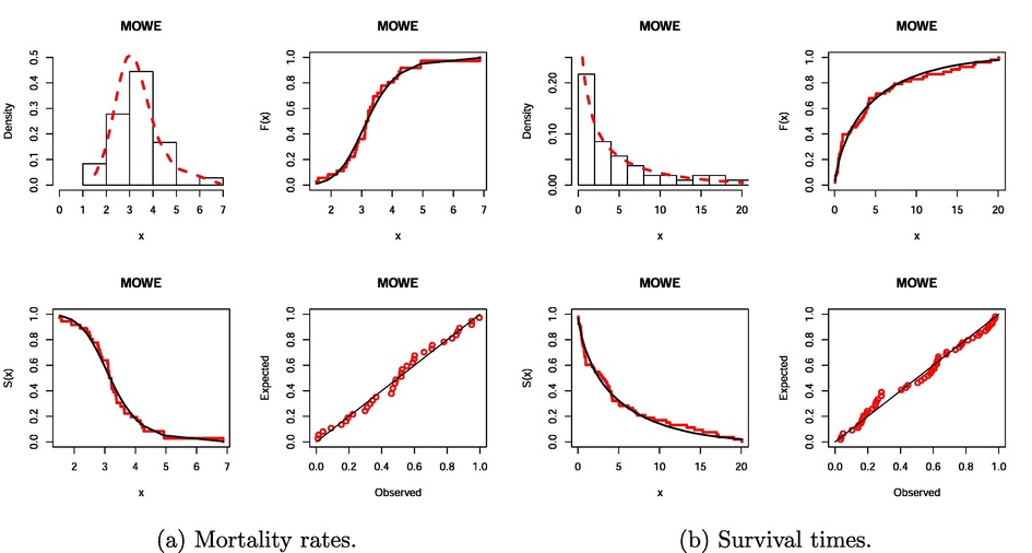
Fitted functions for the MOWE model for the two data sets.

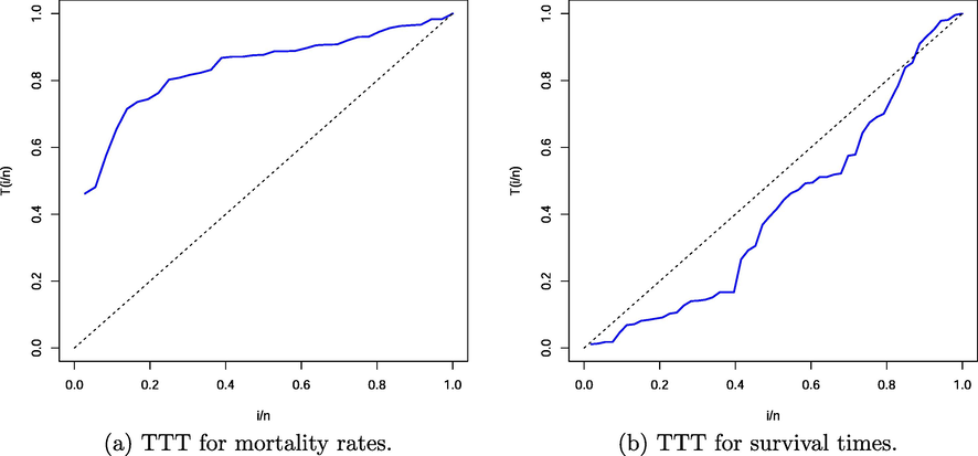
TTT plots for the two analyzed data sets.

7 Concluding remarks

We constructed a new competitive family of distributions to the well-established beta-G and Kumaraswamy-G classes. Some of its mathematical properties were determined. We addressed eight estimation methods for a special model called the MOW-exponential (MOWE) distribution. The simulation results showed that the maximum likelihood approach is the best estimation method for the MOWE parameters. We proved the utility of this distribution to analyze COVID-19 data from Canada and China.

The topics of this article can be extended in several ways. For example, a discrete version of the new family can be established and its properties can be explored. Bivariate extensions of the new family can also be investigated.

Data Availability

This work is mainly a methodological development and has been applied on secondary data, but, if required, data will be provided.

Fund

This study was funded by Taif University Researchers Supporting Project number (TURSP-2020/279), Taif University, Taif, Saudi Arabia.

Declaration of Competing Interest

The authors declare that they have no known competing financial interests or personal relationships that could have appeared to influence the work reported in this paper.

References

Afify A.Z., Al-Mofleh H., Dey S., . Topp–Leone odd log-logistic exponential distribution: Its improved estimators and applications. Anais da Academia Brasileira de Ciências. 2021;93:e20190586
[Google Scholar]
Afify A.Z., Cordeiro G.M., Ibrahim N.A., Jamal F., Elgarhy M., Nasir M.A., . The Marshall-Olkin odd Burr III-G family: theory, estimation, and engineering applications. IEEE Access. 2021;9:4376-4387.
[Google Scholar]
Afify A.Z., Marzouk W., Al-Mofleh H., Ahmed A.H.N., Abdel-Fatah N.A., . The extended failure rate family: properties and applications in the engineering and insurance fields. Pakis. J. Stat.. 2022;38):165-196.
[Google Scholar]
Afify A.Z., Yousof H.M., Alizadeh M., Ghosh I., Ray S., Ozel G., . The Marshall-Olkin transmuted-G family of distributions. Stochast. Qual. Control. 2020;35:79-96.
[Google Scholar]
Al-Babtain A.A., Shakhatreh M.K., Nassar M., Afify A.Z., . A new modified Kies family: properties, estimation under complete and type-II censored samples, and engineering applications. Mathematics. 2020;8:1345.
[Google Scholar]
Alexander C., Cordeiro G.M., Ortega E.M., Sarabia J.M., . Generalized beta-generated distributions. Comput. Stat. Data Anal.. 2012;56:1880-1897.
[Google Scholar]
Bourguignon M., Silva R.B., Cordeiro G.M., . The Weibull-G family of probability distributions. J. Data Sci.. 2014;12:53-68.
[Google Scholar]
Chen Z., . A new two-parameter lifetime distribution with bathtub shape or increasing failure rate function. Stat. Prob. Lett.. 2000;49:155-161.
[Google Scholar]
Cordeiro G.M., Afify A.Z., Ortega E.M., Suzuki A.K., Mead M.E., . The odd Lomax generator of distributions: properties, estimation and applications. J. Comput. Appl. Math.. 2019;347:222-237.
[Google Scholar]
Cordeiro G.M., de Castro M., . A new family of generalized distributions. J. Stat. Comput. Simul.. 2011;81:883-898.
[Google Scholar]
Cordeiro G.M., Lemonte A.J., Ortega E.M., . The Marshall-Olkin family of distributions: mathematical properties and new models. J. Stat. Theory Practice. 2014;8:343-366.
[Google Scholar]
Cordeiro G.M., Ortega E.M., da Cunha D.C., . The exponentiated generalized class of distributions. J. Data Sci.. 2013;11:1-27.
[Google Scholar]
Eugene N., Lee C., Famoye F., . Beta-normal distribution and its applications. Commun. Stat. Theory Methods. 2002;31:497-512.
[Google Scholar]
Gupta R.C., Gupta P.L., Gupta R.D., . Modeling failure time data by Lehman alternatives. Commun. Stat. Theory Methods. 1998;27:887-904.
[Google Scholar]
Hassan A.S., Hemeda S.E., . A new fmily of additive Weibull-generated distributions. Int. J. Math. Appl.. 2017;4:151-164.
[Google Scholar]
Jones M.C., . Families of distributions arising from distributions of order statistics. Test. 2004;13:1-43.
[Google Scholar]
Khan M.S., King R., Hudson I.L., . Transmuted generalized exponential distribution: a generalization of the exponential distribution with applications to survival data. Commun. Stat. Simul. Comput.. 2017;6:4377-4398.
[Google Scholar]
Korkmaz M.C., Cordeiro G.M., Yousof H.M., Pescim R.R., Afify A.Z., Nadarajah S., . The Weibull Marshall-Olkin family: regression model and application to censored data. Commun. Stat. Theory Methods. 2019;8:4171-4194.
[Google Scholar]
Lemonte A.J., Cordeiro G.M., Moreno-Arenas G., . A new useful three-parameter extension of the exponential distribution. Statistics. 2016;50:312-337.
[Google Scholar]
Liu X., Ahmad Z., Gemeay A.M., Abdulrahman A.T., Hafez E.H., Khalil N., . Modeling the survival times of the COVID-19 patients with a new statistical model: a case study from China. PloS One. 2021;16:e0254999
[Google Scholar]
Marshall A.W., Olkin I., . A new method for adding a parameter to a family of distributions with application to the exponential and Weibull families. Biometrika. 1997;84:641-652.
[Google Scholar]
Mead M.E., Afify A.Z., Butt N.S., . The modified Kumaraswamy Weibull Distribution: properties and Applications in Reliability and Engineering Sciences. Pakistan J. Stat. Oper. Res.. 2020;16:433-446.
[Google Scholar]
Nadarajah S., Kotz S., . The exponentiated type distributions. Acta Appl. Math.. 2006;92:97-111.
[Google Scholar]
Nassar M., Afify A.Z., Dey S., Kumar D., . A new extension of Weibull distribution: properties and different methods of estimation. J. Comput. Appl. Math.. 2018;336:439-457.
[Google Scholar]
Nassar M., Kumar D., Dey S., Cordeiro G.M., Afify A.Z., . The Marshall-Olkin alpha power family of distributions with applications. J. Comput. Appl. Math.. 2019;351:41-53.
[Google Scholar]
Nofal Z.M., Afify A.Z., Yousof H.M., Cordeiro G.M., . The generalized transmuted-G family of distributions. Commun. Stat. Theory Methods. 2017;46:4119-4136.
[Google Scholar]
Phani K.K., . A new modified Weibull distribution. Commun. Am. Ceram. Soc.. 1987;70:182-184.
[Google Scholar]
Ramos P.L., Nascimento D.C., Cocolo C., Nicola M.J., Alonso C., Ribeiro L.G., Ennes A., Louzada F., . Reliability-centered maintenance: analyzing failure in harvest sugarcane machine using some generalizations of the Weibull distribution. In: Modelling and Simulation in Engineering, 2018. 2018. p. :1241856.
[Google Scholar]
Ramos P.L., Nascimento D.C., Ferreira P.H., Weber K.T., Santos T.E., Louzada F., . Modeling traumatic brain injury lifetime data: improved estimators for the generalized gamma distribution under small samples. PLoS one. 2019;14:e0221332
[Google Scholar]
Rasekhi M., Alizadeh M., Altun E., Hamedani G.G., Afify A.Z., Ahmad M., . The modified exponential distribution with applications. Pakistan J. Stat.. 2017;33:383-398.
[Google Scholar]
Ristic M.M., Kundu D., . Marshall-Olkin generalized exponential distribution. Metron. 2015;73:317-333.
[Google Scholar]
Rodrigues G.C., Louzada F., Ramos P.L., . Poisson-exponential distribution: different methods of estimation. Journal of Applied Statistics. 2018;45:128-144.
[Google Scholar]
Shaw, W.T., Buckley, I.R., 2007. The alchemy of probability distributions: beyond Gram-Charlier expansions, and a skew-kurtotic-normal distribution from a rank transmutation map, UCL discovery repository. http://discovery.ucl.ac.uk/id/eprint/643923.
Smith R.M., Bain L.J., . An exponential power life testing distribution. Commun. Stat.– Theory Methods. 1975;4:469-481.
[Google Scholar]
Tahir M.H., Nadarajah S., . Parameter induction in continuous univariate distributions: well-established G families. Anais da Academia Brasileira de Ciências. 2015;87:539-568.
[Google Scholar]
Yousof H.M., Afify A.Z., Hamedani G.G., Aryal G.R., . The Burr X Generator of Distributions for Lifetime Data. J. Stat. Theory Appl.. 2017;16:288-305.
[Google Scholar]
Zaidi S.M., Sobhi M.M.A., El-Morshedy M., Afify A.Z., . A new generalized family of distributions: properties and applications. Aims Math.. 2021;6:456-476.
[Google Scholar]
Zografos K., Balakrishnan N., . On families of beta-and generalized gamma-generated distributions and associated inference. Stat. Methodol.. 2009;6:344-362.
[Google Scholar]