The Marshall-Olkin Kappa distribution: Properties and applications

2.1 General theory of Marshall-Olkin distribution

Marshall and Olkin (1997) presented an elastic semi-parametric family of distributions. They defined a new survival function ${\overline{F}}^{\mathit{MO}}(t)$ by inducting an extra parameter $\delta >0$ where $\delta$ was a tilt parameter. They took $\delta$ in the sense of the performance of the hrf of ${\overline{F}}^{\mathit{MO}}(t)$ and the cdf of the baseline distribution. $\delta$ was reintroduced by Nanda and Das (2012) due to the reason that the hrf of the newly introduced distribution is lifted beneath $(\delta 1)$ or overhead $(0<\delta 1)$ the hrf of the original distribution.

The survival function ${\overline{F}}^{\mathit{MO}}(t)$ of MO distribution is $${\overline{F}}^{\mathit{MO}}(t)=\frac{\delta \overline{G}(t)}{1-\overline{\delta }\overline{G}(t)}=\frac{\delta \overline{G}(t)}{G(t)+\delta \overline{G}(t)}\text{or}\frac{\delta [1-G(t)]}{\delta +\overline{\delta }G(t)}$$ where $g(t)\text{,}G(t)\text{and}\overline{G}(t)$ are the pdf, cdf and the survival function of the existing distribution respectively with condition −∞ < t < ∞, $\delta >0$ and $\overline{\delta }=1-\delta$ .

The associated cdf and pdf of MO distribution are

Marshall-Olkin generalizations of different distributions exist in the literature. Some of them are mentioned in our manuscript. Cordeiro and Lemonte (2013) studied the mathematical properties and applications of the Marshall-Olkin extended (MOE) weibull distribution. Other examples include MOE pareto distribution (Alice and Jose, 2003), MOE gamma distribution (Ristić et al., 2007), MOE lomax distribution (Ghitany et al., 2007a), MOE weibull distribution and its application to censored data (Ghitany et al., 2007b), MOE normal distribution (Garcia et al., 2010), MOE lindley distribution (Ghitany et al., 2012), MOE fréchet distribution (Krishna et al., 2013), and MOE birnbaum–saunders distribution (Lemonte, 2013). General properties of the MOE family of distributions were studied recently by Barreto-Souza et al. (2013) and Cordeiro et al. (2014).

3.1 Sub models of MOK distribution

1. In case $\delta =1$ in (3.2), the MOK distribution reduces to KAP-III distribution.

2. If $\theta =\delta =1$ in (3.2), the MOK distribution reduces to KAP-II distribution.

Graphical representation of pdf and cdf for various values of parameters chosen arbitrary are provided in Figs. 3.1 and 3.2 respectively.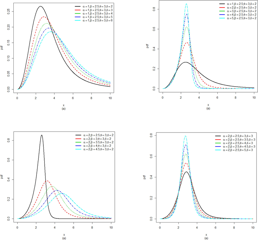

Close

Fig. 3.1

Graphs of the pdf of MOK distribution.

Export to PPT

Close

Fig. 3.2

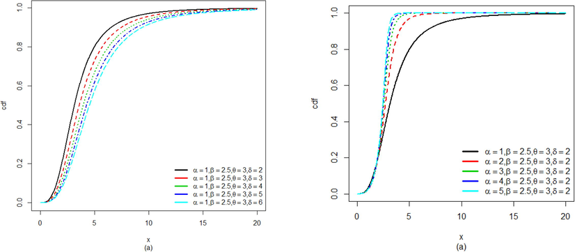
Graphs of the cdf of MOK distribution.

Export to PPT

Some important findings from graphs in Fig. 3.1 are

• The density function of MOK distribution tends to normal distribution as the value of $\delta$ increases, while the values of $\alpha \text{,}\beta \text{and}\theta$ are kept constant. Similar pattern is seen with increase in value of $\beta$ for fixed values of $\alpha \text{,}\theta \text{,}\delta$ .

• $\alpha$ being the shape parameter changes the shape of density function for fixed values of $\beta \text{,}\theta \text{,}\delta$ . Increase in $\alpha$ makes the density function more leptokurtic. Similar behavior is found for increase in $\theta$ , by fixing the values of $\alpha \text{,}\beta \text{and}\delta$ .

From Fig. 3.2, graphs of the cdf of MOK distribution satisfy the following properties.

• $F_{\mathit{MOK}}(x)$ goes to 0 as $x$ gets smaller

• Conversely ${\text{lim}}_{x\to \infty }{F}_{\mathit{MOK}}(x)=1$

• $F_{\mathit{MOK}}(x)$ is non-decreasing.

3.2 Quantiles and moments

The qth quantile of the MOK distribution is

The median, first and third quartiles of MOK distribution are

The $r\text{th}$ moment of MOK random variable $X$ with pdf given in (3.4) is $${\mu }_r^{\prime }={\displaystyle \sum _{k=0}^{\infty }}{W}_k{\beta }^r{\alpha }^{\frac{r}{\alpha \theta }-1}{\int }_0^1{U}^{\frac{k+1}{\alpha }+\frac{r}{\alpha \theta }-1}{[1-U]}^{1-\frac{r}{\alpha \theta }-1}\mathit{dU}$$

Using beta function,

MOK distribution has the following moment generating function and characteristic function

3.3 Mean deviation

The amount of variability in a distribution can be measured up to some extent with the help of totality of deviations about the mean and about the median.

3.4 Reliability properties

Let $t$ be a life time random variable follows MOK $(\alpha \text{,}\beta \text{,}\theta \text{,}\delta )$ distribution. The hazard rate function of MOK distribution, expressed below, is upside-down shaped. Fig. 3.3 shows the graphical representation of the hrf. $$h(t)=\frac{\delta \frac{\alpha \theta }{\beta }{\left(\frac{t}{\beta }\right)}^{\theta -1}{\left(\alpha +{\left(\frac{t}{\beta }\right)}^{\alpha \theta }\right)}^{-\frac{(\alpha +1)}{\alpha }}}{\left[1-{\left[\delta {\left\{\frac{\alpha }{{\left(\frac{t}{\beta }\right)}^{\alpha \theta }}+1\right\}}^{\frac{1}{\alpha }}+(1-\delta )\right]}^{-1}\right]{\left[\delta +(1-\delta ){\left(\frac{{\left(\frac{t}{\beta }\right)}^{\alpha \theta }}{\alpha +{\left(\frac{t}{\beta }\right)}^{\alpha \theta }}\right)}^{\frac{1}{\alpha }}\right]}^2}$$

Close

Fig. 3.3

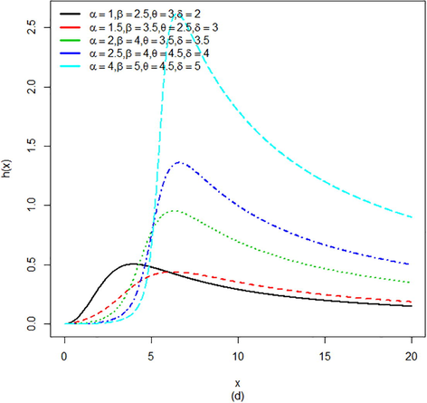
Graph of the hrf of MOK distribution.

Export to PPT

The survival function S(t), cumulative hazard rate function $H(t)$ and reversed hazard rate function $r(t)$ are, respectively, specified as $$S(t)={\left[1+{\left[\delta {\left(\frac{\alpha }{{\left(\frac{t}{\beta }\right)}^{\alpha \theta }}+1\right)}^{\frac{1}{\alpha }}-\delta \right]}^{-1}\right]}^{-1}$$ $$H(t)={\int }_0^{t}h(t)\mathit{dt}=-\mathit{lnS}(t)=-\mathit{ln}\left[1-{\left[\delta {\left\{\frac{\alpha }{{\left(\frac{t}{\beta }\right)}^{\alpha \theta }}+1\right\}}^{\frac{1}{\alpha }}+(1-\delta )\right]}^{-1}\right]$$ and $$r(t)=\frac{f(t)}{F(t)}=\frac{\delta \frac{\alpha \theta }{\beta }{\left(\frac{t}{\beta }\right)}^{\theta -1}{\left(\alpha +{\left(\frac{t}{\beta }\right)}^{\alpha \theta }\right)}^{-\frac{(\alpha +1)}{\alpha }}}{{\left[\delta +(1-\delta ){\left(\frac{{\left(\frac{t}{\beta }\right)}^{\alpha \theta }}{\alpha +{\left(\frac{t}{\beta }\right)}^{\alpha \theta }}\right)}^{\frac{1}{\alpha }}\right]}^2}\left[\delta {\left\{\frac{\alpha }{{\left(\frac{t}{\beta }\right)}^{\alpha \theta }}+1\right\}}^{\frac{1}{\alpha }}+(1-\delta )\right]$$

3.5 Mean residual life function

In many fields like biomedical science, insurance and industrial reliability, mean residual life function is an imperative consideration. It can be obtained through the expression below $$m(t)=\frac{1}{S(t)}\left\{E(t)-{\int }_0^t\mathit{tf}(t)\mathit{dt}\right\}-t$$

Mean residual life function of MOK distribution is given as $$m(t)=\frac{{\sum }_{k=0}^{\infty }{W}_k\beta {\alpha }^{\frac{1}{\alpha \theta }-1}\left\{B\left(\frac{k+1}{\alpha }+\frac{1}{\alpha \theta }\text{,}1-\frac{1}{\alpha \theta }\right)-B_U\left(\frac{k+1}{\alpha }+\frac{1}{\alpha \theta }\text{,}1-\frac{1}{\alpha \theta }\right)\right\}}{1-{\left[\delta {\left\{\frac{\alpha }{{\left(\frac{t}{\beta }\right)}^{\alpha \theta }}+1\right\}}^{\frac{1}{\alpha }}+(1-\delta )\right]}^{-1}}-t$$

3.6 Inequality measures

Inequality measures play key role in many fields like economics to study income and poverty, demography, insurance and medicine. Some are discussed in this study.

3.6.1 An American economist Lorenz (1905) developed a graphical diagram of wealth distribution called Lorenz curve. Lorenz index is defined as $$L(p)=\frac{1}{\mu }{\int }_0^x\mathit{xf}(x)\mathit{dx}$$

The Lorenz curve is the plot of Lorenz index L(p) verses x, given below is the Lorenz index for MOK distribution. $$L(p)=\frac{\beta {\alpha }^{\frac{1}{\alpha \theta }-1}{\sum }_{k=0}^{\infty }{W}_k{B}_U\left(\frac{k+1}{\alpha }+\frac{1}{\alpha \theta }\text{,}1-\frac{1}{\alpha \theta }\right)}{{\sum }_{k=0}^{\infty }{W}_k\beta {\alpha }^{\frac{1}{\alpha \theta }-1}B\left(\frac{k+1}{\alpha }+\frac{1}{\alpha \theta }\text{,}1-\frac{1}{\alpha \theta }\right)}$$

On the diagram perfect equality of wealth distribution is depicted by a straight diagonal line and a line lies under it shows the true wealth distribution. The difference between two above stated lines is actually the inequality of wealth distribution.

3.6.2 A measure of income inequality was projected by Bonferroni (1930), founded on partial means, that is needed when the main source of income inequality is the occurrence of units whose income is much beneath those of others. The Bonferroni index can be determined through the relation $$\mathit{BC}(p)=\frac{L(p)}{F(x)}$$

The Bonferroni curve is the plot of Bonferroni index BC(p) verses $x$ , and this index for MOK distribution is as $$\mathit{BC}(p)=\left[\delta {\left\{\frac{\alpha }{{\left(\frac{x}{\beta }\right)}^{\alpha \theta }}+1\right\}}^{\frac{1}{\alpha }}+(1-\delta )\right]\left[\frac{\beta {\alpha }^{\frac{1}{\alpha \theta }-1}{\sum }_{k=0}^{\infty }{W}_k{B}_U\left(\frac{k+1}{\alpha }+\frac{1}{\alpha \theta }\text{,}1-\frac{1}{\alpha \theta }\right)}{{\sum }_{k=0}^{\infty }{W}_k\beta {\alpha }^{\frac{1}{\alpha \theta }-1}B\left(\frac{k+1}{\alpha }+\frac{1}{\alpha \theta }\text{,}1-\frac{1}{\alpha \theta }\right)}\right]$$

3.6.3 The Zenga index denoted by $Z$ was suggested by Zenga (1984). It measures the disparity between the poorest $p\ast 100\%$ of the population and the wealthier outstanding $(1-p)\ast 100\%$ part of the population by looking at the mean salaries of these two disjoint and comprehensive subpopulations. Zenga index for MOK distribution is as follows $$Z=1-\left[\frac{\left[\beta {\alpha }^{\frac{1}{\alpha \theta }-1}{\displaystyle \sum _{k=0}^{\infty }}{W}_k{B}_U(\frac{k+1}{\alpha }+\frac{1}{\alpha \theta }\text{,}1-\frac{1}{\alpha \theta })\right]\left[\delta {\left\{\frac{\alpha }{{\left(\frac{x}{\beta }\right)}^{\alpha \theta }}+1\right\}}^{\frac{1}{\alpha }}+(1-\delta )\right]}{\left[\mu -\beta {\alpha }^{\frac{1}{\alpha \theta }-1}{\displaystyle \sum _{k=0}^{\infty }}{W}_k{B}_U(\frac{k+1}{\alpha }+\frac{1}{\alpha \theta }\text{,}1-\frac{1}{\alpha \theta })\right]{\left[1-{\left[\delta {\left\{\frac{\alpha }{{(\frac{x}{\beta })}^{\alpha \theta }}+1\right\}}^{\frac{1}{\alpha }}+(1-\delta )\right]}^{-1}\right]}^{-1}}\right]$$

3.6.4 Atkinson (1970) proposed an index ranges from 0 to 1 where 0 means an equal wealth distribution. Mathematically Atkinson index can be defined as $$A_F({\theta }^{\prime }\text{,}∊)=1-\frac{1}{\mu }{\left\{{\int }_0^{\infty }{x}^{1-∊}\mathit{dF}(x)\right\}}^{\frac{1}{1-∊}}$$

Atkinson index for MOK distribution is given by $$A_F({\theta }^{\prime }\text{,}∊)=1-\frac{{\left\{{\sum }_{k=0}^{\infty }{W}_k{\beta }^{1-∊}{\alpha }^{\frac{1-∊}{\alpha \theta }-1}B\left(\frac{k+1}{\alpha }+\frac{1-∊}{\alpha \theta }\text{,}1-\frac{1-∊}{\alpha \theta }\right)\right\}}^{\frac{1}{1-∊}}}{\beta {\alpha }^{\frac{1}{\alpha \theta }-1}{\sum }_{k=0}^{\infty }{W}_{k}B\left(\frac{k+1}{\alpha }+\frac{1}{\alpha \theta }\text{,}1-\frac{1}{\alpha \theta }\right)}$$

3.6.5 Pietra (1915) offered an index, known as Schutz index or half of the relative mean deviation. Pietra index is defined as $$P_X=\frac{1}{2\mu }{\int }_0^{\infty }|x-\mu |\mathit{dF}(x)=\frac{{\mathit{MD}}_{\overline{x}}}{2\mu }$$

Expression for the Pietra index $P_X$ for MOK distribution is $$P_X=\frac{\left[\mu F(\mu )-\beta {\alpha }^{\frac{1}{\alpha \theta }-1}{\sum }_{k=0}^{\infty }{W}_k{B}_U\left(\frac{k+1}{\alpha }+\frac{1}{\alpha \theta }\text{,}1-\frac{1}{\alpha \theta }\right)\right]}{{\sum }_{k=0}^{\infty }{W}_k\beta {\alpha }^{\frac{1}{\alpha \theta }-1}B\left(\frac{k+1}{\alpha }+\frac{1}{\alpha \theta }\text{,}1-\frac{1}{\alpha \theta }\right)}$$

3.7 Generalized entropy (GE)

Variation of the uncertainty can be measured for a random variable through entropy. The generalized entropy (GE) index, suggested by Cowell (1980) and Shorrocks (1980) is $${\mathit{GE}}_F({\theta }^{\prime }\text{,}\omega )=\frac{1}{\omega (\omega -1)}\left\{\frac{{\mu }_{\omega }^{\prime }}{{\mu }^{\omega }}-1\right\}$$ where ${\mu }_{\omega }^{\prime }$ is the $\omega \mathit{th}$ moment about origin.

The GE for MOK distribution can be obtained as below $${\mathit{GE}}_F\left({\theta }^{\prime }\text{,}\omega \right)=\frac{1}{\omega (\omega -1)}\left\{\frac{{\sum }_{k=0}^{\infty }{W}_k{\beta }^{\omega }{\alpha }^{\frac{\omega }{\alpha \theta }-1}B\left(\frac{k+1}{\alpha }+\frac{\omega }{\alpha \theta }\text{,}1-\frac{\omega }{\alpha \theta }\right)}{{\left({\sum }_{k=0}^{\infty }{W}_k\beta {\alpha }^{\frac{1}{\alpha \theta }-1}B\left(\frac{k+1}{\alpha }+\frac{1}{\alpha \theta }\text{,}1-\frac{1}{\alpha \theta }\right)\right)}^{\omega }}-1\right\}$$

3.8 Order statistics

In many areas of statistical theory and applications, order statistics have significant role. Consider $X_1\text{,}\dots \text{,}{X}_n$ is a random sample from a population with the MOK $(\alpha \text{,}\beta \text{,}\theta \text{,}\delta )$ distribution. Let $X_{i\text{,}n}$ denote the $\mathit{ith}$ order statistics then its pdf is given as $$f_{i\text{,}n}(x)=\frac{n!}{(i-1)!(n-i)!}f(x)F{(x)}^{i-1}{\{1-F(x)\}}^{n-i}$$

Inserting pdf and cdf of Kappa distribution and simplifying we get $$f_{i\text{,}n}(x)=\frac{n!}{(i-1)!(n-i)!}{\displaystyle \sum _{j=0}^{n-i}}{\displaystyle \sum _{k=0}^{\infty }}{(-1)}^j\left(\begin{array}{c}\hfill n-i\hfill \\ \hfill j\hfill \end{array}\right)W_k\left(\frac{\alpha \theta }{\beta }\right){\left(\frac{x}{\beta }\right)}^{\theta -1}{\left[\alpha +{\left(\frac{x}{\beta }\right)}^{\alpha \theta }\right]}^{-\frac{\alpha +1}{\alpha }}\times {\left[\frac{{(\frac{x}{\beta })}^{\alpha \theta }}{\alpha +{\left(\frac{x}{\beta }\right)}^{\alpha \theta }}\right]}^{\frac{k}{\alpha }}{\left[\delta {\left\{\frac{\alpha }{{\left(\frac{x}{\beta }\right)}^{\alpha \theta }}+1\right\}}^{\frac{1}{\alpha }}+(1-\delta )\right]}^{(1-j-i)}$$

3.9 Estimation of parameters

Section given below considers the famous and most useful method for estimating the parameters $\alpha \text{,}\beta \text{,}\theta \text{and}\delta$ of MOK distribution. Let $X\sim \text{MOK}(\alpha \text{,}\beta \text{,}\theta \text{,}\delta )$ distribution. We estimate these parameters with the help of method of maximum likelihood. Consider the log-likelihood function $\ell =L(\mathrm{\Theta })$ $$\ell =\mathit{nlog}(\delta \alpha \theta )-\mathit{nlog}\beta +(\theta -1){\displaystyle \sum _{i=1}^n}\mathit{log}\left(\frac{x_i}{\beta }\right)-\left(\frac{\alpha +1}{\alpha }\right){\displaystyle \sum _{i=1}^n}\mathit{log}\left[\alpha +{\left(\frac{x_i}{\beta }\right)}^{\alpha \theta }\right]-2{\displaystyle \sum _{i=1}^n}\mathit{log}\left\{\delta +(1-\delta ){\left[\alpha {\left(\frac{x_i}{\beta }\right)}^{-\alpha \theta }+1\right]}^{-\frac{1}{\alpha }}\right\}$$

Partially differentiating $\ell$ with respect to $\alpha \text{,}\beta$ , $\theta \mathit{and}\delta$ and then equate to zero,

We have four equations as $$\frac{\partial \ell }{\partial \alpha }=\frac{n}{\alpha }-\left(\frac{\alpha +1}{\alpha }\right){\displaystyle \sum _{i=1}^n}\left[{\left[\alpha +{\left(\frac{x_i}{\beta }\right)}^{\alpha \theta }\right]}^{-1}\left[1+{\left(\frac{x_i}{\beta }\right)}^{\alpha \theta }\right]\log \left(\frac{x_i}{\beta }\right)\right]+\frac{1}{{\alpha }^2}{\displaystyle \sum _{i=1}^n}\mathit{log}\left[\alpha +{\left(\frac{x_i}{\beta }\right)}^{\alpha \theta }\right]-2{\displaystyle \sum _{i=1}^n}\frac{\left(1-\delta \right)\left[\alpha +{\left(\frac{x_i}{\beta }\right)}^{\alpha \theta }\right]\mathit{log}\left[\alpha {\left(\frac{x_i}{\beta }\right)}^{-\alpha \theta }+1\right]+\log \left(\frac{x_i}{\beta }\right){\alpha }^2\theta -\alpha }{\left[\delta +\left(1-\delta \right){\left[\alpha {\left(\frac{x_i}{\beta }\right)}^{-\alpha \theta }+1\right]}^{-\frac{1}{\alpha }}\right]{\left[\alpha {\left(\frac{x_i}{\beta }\right)}^{-\alpha \theta }+1\right]}^{\frac{1}{\alpha }}{\alpha }^2\left[\alpha +{\left(\frac{x_i}{\beta }\right)}^{\alpha \theta }\right]}=0$$ $$\frac{\partial \ell }{\partial \beta }=-\frac{n}{\beta }-\left(\frac{\theta -1}{\beta }\right)+\frac{(\alpha +1)\theta }{\beta }{\displaystyle \sum _{i=1}^n}\left[{\left[\alpha +{\left(\frac{x_i}{\beta }\right)}^{\alpha \theta }\right]}^{-1}{\left(\frac{x_i}{\beta }\right)}^{\alpha \theta }\right]+\frac{2(1-\delta )\theta }{\beta }{\displaystyle \sum _{i=1}^n}\left[{\left\{\delta +(1-\delta ){\left[\alpha {\left(\frac{x_i}{\beta }\right)}^{-\alpha \theta }+1\right]}^{-\frac{1}{\alpha }}\right\}}^{-1}{\left[\alpha {\left[\frac{x_i}{\beta }\right]}^{-\alpha \theta }+1\right]}^{-\frac{1}{\alpha }-1}{\left(\frac{x_i}{\beta }\right)}^{-\alpha \theta }\right]=0$$ $$\frac{\partial \ell }{\partial \theta }=\frac{n}{\theta }+{\displaystyle \sum _{i=1}^n}\mathit{log}\left(\frac{x_i}{\beta }\right)-(\alpha +1){\displaystyle \sum _{i=1}^n}\left[\frac{{\left(\frac{x_i}{\beta }\right)}^{\alpha \theta }\mathit{log}\left(\frac{x_i}{\beta }\right)}{\alpha +{\left(\frac{x_i}{\beta }\right)}^{\alpha \theta }}\right]+2\alpha (1-\delta )\times {\displaystyle \sum _{i=1}^n}\left[{\left\{\delta +(1-\delta ){\left[\alpha {\left(\frac{x_i}{\beta }\right)}^{-\alpha \theta }+1\right]}^{-\frac{1}{\alpha }}\right\}}^{-1}{\left[\alpha {\left(\frac{x_i}{\beta }\right)}^{-\alpha \theta }+1\right]}^{-\frac{1}{\alpha }-1}{\left(\frac{x_i}{\beta }\right)}^{-\alpha \theta }\mathit{log}\left(\frac{\alpha x_i}{\beta }\right)\right]=0$$ $$\frac{\partial \ell }{\partial \delta }=\frac{n}{\delta }-2{\displaystyle \sum _{i=1}^n}\left[{\left\{\delta +(1-\delta ){\left[\alpha {\left(\frac{x_i}{\beta }\right)}^{-\alpha \theta }+1\right]}^{-\frac{1}{\alpha }}\right\}}^{-1}\left[1-{\left\{\alpha {\left(\frac{x_i}{\beta }\right)}^{-\alpha \theta }+1\right\}}^{-\frac{1}{\alpha }}\right]\right]=0$$ Hence, the MLEs of $\alpha \text{,}\beta \text{,}\theta \mathit{and}\delta$ for MOK distribution can be obtained by solving above equations. This task can be successfully done with any statistical package for example R.

4.1 On stream flow amounts (1000 acre-feet)

Following data set (Mielke and Johnson, 1973) consists of stream flow amounts (1,000 acre-feet) for 35 years (1936–70) at the U.S. Geological Survey (USGS) gaging station number 9–3425 for 1st April to 31st August of each year.

192.48, 303.91, 301.26, 135.87, 126.52, 474.25, 297.17, 196.47, 327.64, 261.34, 96.26, 160.52, 314.60, 346.30, 154.44, 111.16, 389.92, 157.93, 126.46, 128.58, 155.62, 400.93, 248.57, 91.27, 238.71, 140.76, 228.28, 104.75, 125.29, 366.22, 192.01, 149.74, 224.58, 242.19, 151.25.

4.2 On failure times of mechanical components

Following data represents the failure times of mechanical components obtained from Silva et al. (2015).

0.040, 1.866, 2.385, 3.443, 0.301, 1.876, 2.481, 3.467, 0.309, 1.899, 2.610, 3.478, 0.557, 1.911, 2.625, 3.578, 0.943, 1.912, 2.632, 3.595, 1.070, 1.914, 2.646, 3.699, 1.124, 1.981, 2.661, 3.779, 1.248, 2.010, 2.688, 3.924, 1.281, 2.038, 2.823, 4.035, 1.281, 2.085, 2.890, 4.121, 1.303, 2.089, 2.902, 4.167, 1.432, 2.097, 2.934, 4.240, 1.480, 2.135, 2.962, 4.255, 1.505, 2.154, 2.964, 4.278, 1.506, 2.190, 3.000, 4.305, 1.568, 2.194, 3.103, 4.376, 1.615, 2.223, 3.114, 4.449, 1.619, 2.224, 3.117, 4.485, 1.652, 2.229, 3.166, 4.570, 1.652, 2.300, 3.344, 4.602, 1.757, 2.324, 3.376, 4.663

Tables 4.1 and 4.2 present the maximum likelihood estimates of the parameters of the distributions and their standard errors in parenthesis. Table 4.3 shows the minimum values of the log likelihood function $\ell (·)$ and performance indices $W^{\ast }$ and $A^{\ast }$ for all the distributions under study on both data sets. It is worth pointing that MOK distribution has smallest values of $W^{\ast }$ and $A^{\ast }$ as compared to the rest distributions. Fig. 4.1 depicts the graphical representation of fitness of MOK and other forms of kappa distribution. It is evident from performance indices and graph that MOK is the good fit distribution for both data sets so it can be considered that the proposed model is a good competitive model.

Close

Fig. 4.1

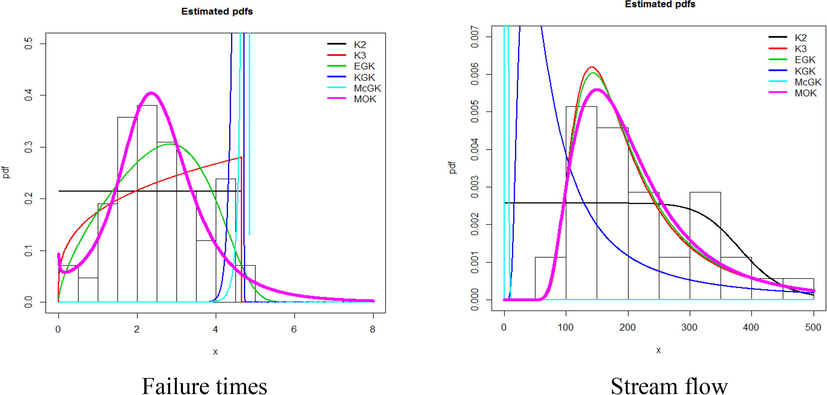
Graphs of the estimated pdfs for G-Kappa distributions.

Export to PPT

References

- General results for the Marshall and Olkin’s family of distributions. Ann. Braz. Acad. Sci.. 2013;85:3-21.
- [Google Scholar]
- Elementi di statistica generale. Firenze: Libreria Seber; 1930.
- The Marshall-Olkin family of distributions: mathematical properties and new models. J. Stat. Theor. Pract.. 2014;8:343-366.
- On the structure of additive inequality measures. Rev. Econ. Stud.. 1980;47:521-531.
- A new skew generalization of the normal distribution: properties and applications. Comput. Stat. Data. An.. 2010;54:2021-2034.
- Marshall-Olkin extended Lomax distribution and its application to censored data. Commun. Stat-Theor. M.. 2007;36:1855-1866.
- Marshall-Olkin extended Weibull distribution and its application to censored data. J. Appl. Stat.. 2007;32:1025-1036.
- Marshall-Olkin extended Lindley distribution and its application. Int. J. Ap. Mat.. 2012;25:709-721.
- Hussain, S., 2015. Extension, Properties and Application of Kappa Distribution. M.Phil. Thesis, Submitted to Government College University, Faisalabad, Pakistan. (Unpublished).
- The Marshall-Olkin Fréchet distribution. Commun. Stat-Theor. M.. 2013;42:4091-4107.
- A new extension of the Birnbaum-Saunders distribution. Braz. J. Probab. Stat.. 2013;27:133-149.
- Method of measuring the concentration of wealth. J. Am. Stat. Assoc.. 1905;9:209-219.
- A new method for adding a parameter to a family of distributions with application to the exponential and Weibull families. Biometrika.. 1997;84:641-652.
- Another family of distributions for describing and analyzing precipitation data. J. Appl. Meteorol.. 1973;12(2):275-280.
- Three parameter kappa distribution maximum likelihood estimations and likelihood ratio tests. Mon. Weather Rev.. 1973;101:701-707.
- Stochastic orders of the Marshall-Olkin extended distribution. Stat. Probabil. Lett.. 2012;82:295-302.
- The new class of Kummer beta generalized distributions. SORT-Stat. Oper. Res. T.. 2012;36:153-180.
- Delle relazioni fra indici di variabilita, note I e II. Atti del Reale Istituto Veneto di scienze. Lettere ed Arti.. 1915;74:775-804.
- A Marshall-Olkin gamma distribution and minification process. STARS: Stress and Anxiety Research. Society.. 2007;11:107-117.
- A new extended gamma generalized model. Int. J. Pure Appl. Math... 2015;100(2):309-335.
- The Class of additively decomposable inequality measures. Econometrica.. 1980;48:613-625.
- Proposta per un indice di concentrazione basto sui rapporti fra quantili di populizone e quantili ti reddito. Giornale degli economisti e Annali di Economia. 1984;48:301-326.