Quintic non-polynomial spline methods for third order singularly perturbed boundary value problems

1 Introduction

Any differential equation whose solution changes rapidly in some parts of the interval or domain is known as singular perturbation problem. These problems arise very frequently in diversified fields of applied mathematics and engineering, for instance in fluid mechanics hydrodynamics, quantum mechanics, chemical-reactor theory, aerodynamics, plasma dynamics, rarefied-gas dynamics, oceanography, meteorology, modeling of semiconductor devices, diffraction theory and reaction–diffusion processes and many other allied areas. The numerical solution of perturbed differential equation of the form of self-adjoint second order two point boundary value problems has been presented using the methods such as optimal quadratic and cubic spline collocation on non-uniform partitions (Christara and Ng, 2006), a fourth order adaptive collocation approach and patching approach (Khuri and Sayfy, 2012, 2014). Parametric Quintic and non-polynomial Quintic spline solutions have been presented for third-order boundary value problems and for the system of third order boundary value problems respectively (Khan and Sultana, 2012a,b).

A singular perturbation problem is said to be reaction diffusion type problem, if the order of differential equation is reduced by two (Phaneendral et al. 2012). Basically, the problem of ineffectiveness for solving singularly perturbed problems has been associated with the perturbation parameter. Accordingly, more efficient and simpler numerical methods are required to solve singularly perturbed two-point boundary value problems. In recent years, a large number of methods have been established to provide accurate results (Temsah, 2008; Rashidinia et al., 2007; Jalilian et al., 2015; Reza and Rashidinia, 2009; Ghazala, 2012, 2015; Ghazala and Imran, 2014; Sonali and Hradyesh, 2015). Those shows that a considerable amount of work has been done for the development of numerical methods to boundary value problems using various splines, yet there is lack of accuracy and convergence because the treatment of singular perturbation problems is not trivial distribution and the solution profile depends on perturbation parameter and mesh size h, (Doolan et al., 1980). It is necessary to develop efficient and accurate numerical methods for third order singularly perturbed problems. So,the purpose of this study is to develop a new spline method for the solution of third order singularly perturbed boundary value problem which is more accurate than the existing methods. This method depends on a non-polynomial spline function which has a trigonometric part and a polynomial part.

2 Description of the method

Consider the third order self adjoint singularly perturbed boundary value problem of the form:

The spline function we propose has a form $T_5=\mathit{span}\{1\text{,}x\text{,}{x}^2\text{,}{x}^3\text{,}\mathit{cos}(\mathit{kx})\text{,}\mathit{sin}(\mathit{kx})\}$ where k is the frequency of trigonometric part of the splines function which can be real or imaginary and will be used to raise the accuracy of the method.

For each segment $[x_i\text{,}{x}_{i+1}]\text{,i}=0\text{,}1\text{,}\dots \text{,}n-1$ , the non-polynomial $S_{\mathrm{\Delta }}(x)$ has the following form:

Let $y(x)$ be the exact solution of Eq. (1) with boundary conditions Eq. (2) and $S_i$ be an approximation to $y_i=y(x)$ obtained by the spline function $S_{\mathrm{\Delta }}(x)$ passing through the points $(x_i\text{,}{S}_{\mathrm{\Delta }})\text{and}(x_{i+1}\text{,}{S}_{\mathrm{\Delta }+1})\text{.}$ Following the technique of (Srivastava and Kumar, 2011):

The coefficients in Eq. (3) using Eq. (4) are determined as: $$\begin{array}{c}{a}_i=\frac{F_i}{k^4}\text{,}{b}_i=\frac{F_{i+1}-F_i\cos (\theta )}{k^4\sin (\theta )}\text{,}{c}_i=\frac{D_{i+1}-D_i}{6h}+\frac{F_{i+1}-F_i}{6{\mathit{hk}}^2}\text{,}{d}_i=\frac{1}{2}(D_i+\frac{F_i}{k^2})\hfill \\ e_i=\frac{y_{i+1}-y_i}{h}+\frac{F_i-F_{i+1}}{{\mathit{hk}}^4}-\frac{h}{6}(D_{i+1}+2D_i)-\frac{h}{6k^2}(F_{i+1}+2F_i)\hfill \\ f_i=y_i-\frac{F_i}{k^4}\text{;}\text{for}\text{i}=0\text{,}1\text{,}\dots \text{,n}-1\text{and}\theta =\mathit{kh}\text{.}\hfill \end{array}$$

Applying the first and second derivative continuity at knots, that is, $S_{\mathrm{\Delta }-1}^{(m)}(x_i)=S_{\mathrm{\Delta }}^{(m)}(x_i)$ , for $m=1\text{,}3$ , the following relations are derived:

Subtracting Eq. (6) from Eq. (5), we obtain:

We define the operator $\wedge$ by $\wedge w\equiv p(w_{i+2}+w_{i-2})+{\mathit{sw}}_i+q(w_{i+1}+w_{i-1})$ for any function $w$ evaluated at the mesh points. On applying this operator for $\text{T}$ in Eq. (8), (Kumar and Srivastava, 2009), we have:

Substituting Eq. (8) into Eq. (9), we derive the following useful relation:

Using Eqs. (9) and (10) we obtain:

Rearranging Eq. (1) and evaluating at ‘xi’ we have:

Substituting Eq. (12) into Eq. (11) and simplifying we obtain:

End conditions:

The system in Eq. (13) gives $(n-3)$ linear algebraic equations in the $(n-1)$ unknowns $y_i$ , for $\text{i}=1\text{,}2\text{,}\dots \text{n}-1\text{,}$ So we need two more equations, at each ends. Following the procedure given by Reza and Rashidina (2009), the required end condition can be written as:

For $l=0\text{,}1\text{,}\dots n$ . Eqs. (14) and (15) can be written as:

Expanding each terms of Eq. (16) by Taylor’s series about $x_0$ . then, substituting and collecting coefficients of the same order we obtain:

Expanding Eq. (13) in Taylor’s series about $x_i$ , we obtain the following local truncation error:

Similarly, we can expand each term for Eq. (17), substituting and collecting coefficients of the same order.

Using Eq. (19) and eliminating the coefficients of various powers of h for different choices of parameters $\alpha \text{,}\beta \text{,}p\text{,}q$ and $s$ , where $\alpha +\beta =\frac{1}{2}$ ,

And truncating the terms in Eq. (19) that contains $h^7$ and above, for arbitrary $\alpha$ and $\beta$ provided that $\alpha +\beta =\frac{1}{2}$ , the value of $p\text{,}q$ and $s$ are evaluated from: $$\left\{\begin{array}{c}\hfill 2p+2q+s=1\hfill \\ \hfill 120p+30q=7.5\hfill \\ \hfill 1680p+105q=31.5\hfill \end{array}\right.\text{;}\text{we obtain}:(\alpha \text{,}\beta \text{,}p\text{,}q\text{,}s)=\left(\frac{1}{6}\text{,}\frac{1}{3}\text{,}\frac{1}{240}\text{,}\frac{7}{30}\text{,}\frac{21}{40}\right)$$

After equating each coefficient of orders of Eq. (18) with 0 we obtain the values of parameters

In a similar manner we obtain parameters of the other end condition as:

Using Eqs. (20) and (21) in Eq. (16) and (17) respectively, with the help of Eq. (12) we obtain the two end conditions as:

Hence, Eqs. (13), (22) and (23) gives penta - diagonal system for $i=1\text{,}2\text{,}\dots \text{,}n-1$ and can easily be solved using Gauss-Elimination method.

3 Convergence analysis of the method

Consider the system of Eqs. (11), (22) and (23) in the matrix form as:

The exact solution is defined as $\overline{y}=(y(x_1)\text{,}y(x_2)\text{,}\dots \text{,}y(x_{n-1}))$ , Eq. (24) is written as

To determine the error bounds the row sums, $s_1\text{,}{s}_2\text{,}\dots \text{,}{s}_{n-1}$ of the matrix $A$ are calculated $$s_1={\displaystyle \sum _{j=1}^{n-1}}{a}_{1j}=-320\epsilon -104{\mathit{uh}}^3$$ $$s_2={\displaystyle \sum _{j=1}^{n-1}}{a}_{2j}=-0.5\epsilon -\frac{1314}{1805}{\mathit{uh}}^3$$ $$s_i={\displaystyle \sum _{j=1}^{n-1}}{a}_{\mathit{ij}}=-\frac{41}{56}{\mathit{uh}}^3\text{for}i=3\text{,}\dots \text{,}n-3$$ $$s_{n-2}={\displaystyle \sum _{j=1}^{n-1}}{a}_{n-2j}=0.5\epsilon -\frac{1314}{1805}{\mathit{uh}}^3$$ $$s_{n-1}={\displaystyle \sum _{j=1}^{n-1}}{a}_{n-1j}=-120\epsilon -120{\mathit{uh}}^3$$

Since $0<\epsilon 1$ , we can choose h sufficiently small so that the matrix $A$ is irreducible and monotone. Using, Ghazala (2012) and Mohanty and Jha (2005), it follows that $A^{-1}$ exists and its elements are non-negative. Hence, from Eq. (27), we get $E=A^{-1}T$

Also from the theory of matrices $A^{-1}A=I_{(n-1)\times (n-1)}$

Since each row of sum of matrix is $I_{(n-1)\times (n-1)}=1$ and $A^{-1}A=1$ .

That is $a_{11}^{-1}(a_{11}+a_{12}+\dots a_{1\text{,}n-1})+a_{12}^{-1}(a_{21}+a_{21}+\dots a_{2\text{,}n-1})+\dots +a_{1\text{,}n-1}^{-1}(a_{n-1\text{,}1}+a_{n-1\text{,}2}+\dots a_{n-1\text{,}n-1})=1$

$\Rightarrow a_{11}^{-1}(s_1)+a_{12}^{-1}(s_2)+\dots a_{n-1}^{-1}(s_{n-1})=1$

This is written in a compact form

Defining $S_j=\text{min}{s}_i\text{,}$ from Eq. (29) $$S_j(a_{k\text{,}1}^{-1}+a_{k\text{,}2}^{-1}+\dots +a_{k\text{,}n-1}^{-1})⩽1$$

It follows that

From Eq. (27), the error terms can be written as

Using Eqs. (26) and (30) $$\begin{array}{c}\hfill |e_k|⩽\mathit{max}‖\frac{1}{h^3{B}_{\mathit{io}}}‖{‖\frac{7}{288}\epsilon h^7{y}^{(7)}(\phi )‖}_{\text{,}{x}_{i-2}<(\phi )<x_{i+2}}⩽\frac{1}{h^3{B}_i}\left(\frac{7\epsilon h^7}{288}\right)\mathit{max}{‖y^{(7)}(\phi )‖}_{\text{,}{x}_{i-2}<(\phi )<x_{i+2}}\hfill \\ \hfill |e_k|⩽(\mu \epsilon h^4)\mathit{max}{‖y^{(7)}(\phi )‖}_{\text{,}{x}_{i-2}<(\phi )<x_{i+2}}\text{for j}=1\text{,}2\text{,}\dots \text{,}\text{n}-1\hfill \end{array}$$ where $\mu$ is a constant and independent of h, and hence it follows that $\Vert E\Vert =O(h^4)\text{.}$

This result can be summarized in the following theorem.

4 Numerical examples and results

To demonstrate the validity of the methods, two model singularly perturbed problems have been considered. These examples have been chosen because they have been widely discussed in the literature and their exact solutions were available for comparison.

The analytic solution is $y(x)=6x^3\epsilon {(1-x)}^5$

The numerical solutions in terms of maximum absolute errors are given in Tables 1 and 3 with its graph in Figs. 1 and 2 as follows:

Close

Figure. 1

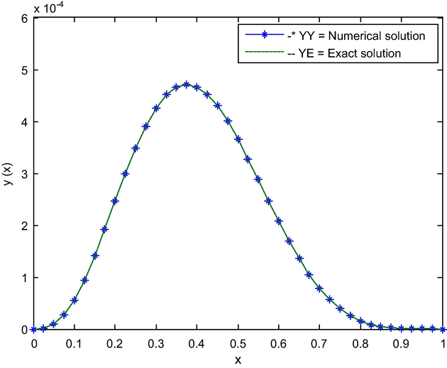
The graph of exact and numerical solution of Example 1 for N = 40 and $\epsilon =\frac{1}{64}$ .

Export to PPT

Close

Figure. 2

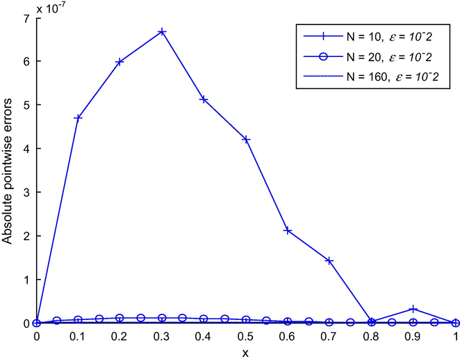
Absolute errors decrease as the Number of mesh N increases for Example 1.

Export to PPT

The numerical results in terms of maximum absolute errors are tabulated in Tables 2 and 3 with its graph given in Fig. 3 and 4.

Close

Figure. 3

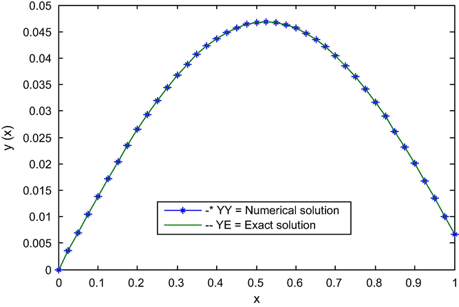
The graph of exact and numerical solution of Example 2 for N = 40 and $\epsilon =\frac{1}{64}$ .

Export to PPT

Close

Figure. 4

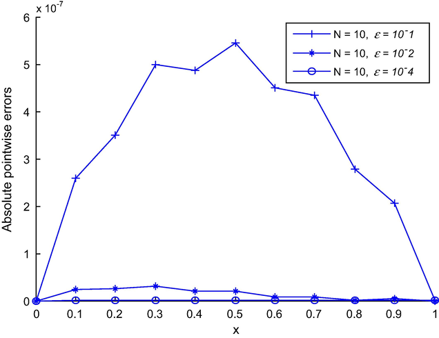
Absolute errors decrease as perturbation parameter $\epsilon$ decreases for Example 2.

Export to PPT

5 Discussion and conclusion

In this paper, the quintic non-polynomial spline method has been presented for solving third order singularly perturbed boundary value problems of the reaction–diffusion equation type. First, the given domain is discretized and the derivative of the given differential equation is replaced by the spline approximations. Then, the system is transformed to penta-diagonal system, which can easily be solved using any appropriate methods for solving the systems of linear equations. To validate the applicability of the proposed method, two model examples have been considered and solved for different values of perturbation parameter and different mesh sizes. The order of convergence has been established for the method and is convergent to order four. As it can be observed from the numerical results presented in Tables 1–3 and graphs (Figs 1 and 3), the present method approximates the exact solution very well. Moreover, the method has been analyzed by taking sufficiently small size of h and perturbation parameter where other existing numerical methods reported in the literature may fail.

The results obtained by the present method have been compared with the numerical results obtained by (Ghazala, 2012; Ghazala and Imran, 2014; and Sonali and Hradyesh, 2015) and is observed to be more accurate than the methods proposed by the aforementioned scholars. Furthermore, the absolute errors decrease rapidly as N increases and the perturbation parameter decreases (Figs. 2 and 4). This method can be extended to higher order Quintic non-polynomial spline methods for solving similar problems.

References

- Optimal quadratic and cubic spline collocation on nonuniform partitions. Computing. 2006;76:227-257. Digital Object Identifier (DOI)
- [CrossRef] [Google Scholar]
- Uniform Numerical Methods for Problems with Initial and Boundary Layers. Dublin: Boole Press; 1980.
- Quartic spline solution of third order singularly perturbed boundary value problem. Anzaim J.. 2012;53 No. E. pp. E44-E58
- [Google Scholar]
- Solution of the system of fifth order boundary value problem using sextic spline. J. Egypt. Math. Soc.. 2015;23(2):406-409.
- Quartic non-polynomial spline solution of third order singularly perturbed boundary value problem. Res. J. Appl. Sci. Eng. Technol.. 2014;7(23):4859-4863.
- Non-polynomial spline for the numerical solution of problems in calculus of variations. Int. J. Math. Model. Comput.. 2015;5(1):1-14.
- Non-polynomial quintic spline solution for the system of third order boundary-value problems. Numer. Algorithm. 2012;59:541-559.
- Parametric quintic spline solution of third-order boundary value problems. Int. J. Comput. Math.. 2012;89(12):1663-1677.
- The boundary layer problem: a fourth -- order adaptive collocation approach. Comput. Math. Appl.. 2012;64(6):2089-2099.
- Self-adjoint singularly perturbed second order two – point boundary value peoblems: a patching approach. Appl. Math. Model.. 2014;38(11):2901-2914.
- Computational techniques for solving differential equations cubic, quintic and sextic spline. Comput. Methods Eng. Sci. Mech.. 2009;10(1):108-115.
- Class of variable mesh spline in compression methods for singularly perturbed two-point singular boundary-value problems. Appl. Math. Comput.. 2005;168(1):704-716.
- Asymptotic-numerical method for third-order singular perturbation problems. Int. J. Appl. Sci. Eng.. 2012;10(3):241-248.
- Spline approach to the solution of a singularly-perturbed boundary-value problems. Appl. Math. Comput.. 2007;189:72-78.
- Non-polynomial spline solution of fourth-order obstacle boundary value problems. Int. J. Math. Comput. Phys. Electr. Comput. Eng.. 2009;3(4):241-247.
- A new quartic B-spline method for third–order self-adjoint singularly perturbed boundary value problems. Appl. Math. Sci.. 2015;9(8):399-408.
- Numerical treatment of non-linear third order boundary value problem. Appl. Math.. 2011;2(8):959-964.
- Spectral methods for some singularly perturbed third order ordinary differential equations. Numer. Algorithm. 2008;47:63-80.