Pattern analysis of protein images from fluorescence microscopy using Gray Level Co-occurrence Matrix

2.1 Datasets

Three benchmark protein image datasets have been utilized to assess the performance of our proposed method. These include 2D HeLa (Boland and Murphy, 2001), CHO (Lin et al., 2007), and LOCATE Endogenous (Nanni et al., 2010a) datasets. The cells in HeLa dataset, comprised of 862 images, are distributed in 10 different classes including Actin Filaments, Endosome, Endoplasmic Reticulum, Golgi Giantin, Golgi GPP130, Lysosome, Microtubules, Mitochondria, Nucleolus, and Nucleus. CHO dataset seizes 668 protein images categorized in 8 unique classes, which include Actin, Endoplasmic Reticulum, Golgi, Microtubule, Mitochondria, Nucleolus, Nucleus, and Peroxisome. The third dataset, LOCATE Endogenous contains 502 protein images and comprised of 10 classes, which are Actin, Endosome, Endoplasmic Reticulum, Golgi, Lysosome, Microtubule, Mitochondria, Nucleus, Peroxisome, and Plasma Membrane.

2.2 The proposed prediction system

Fig. 1 demonstrates the proposed GLCM-SubLoc prediction system. The input image is first quantized to the required number of gray levels. Then for a particular value of offset parameter d, a GLCM is constructed along four directions: horizontal, vertical, diagonal, and off-diagonal as shown in Fig. 2. Next, features are extracted from each of the four GLCMs separately. Then features from horizontal GLCM are averaged with the features from vertical directional GLCM. Similarly, the features from diagonal GLCM are averaged with the features from off-diagonal GLCM. The final feature space is constructed by concatenating the two averaged feature spaces.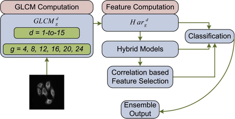

Close

Figure 1

The proposed GLCM-SubLoc prediction system.

Export to PPT

Close

Figure 2

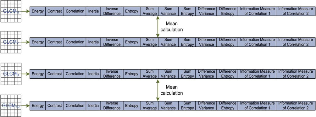
Feature vectors for GLCM along four different directions including: horizontal, vertical, diagonal, and off-diagonal.

Export to PPT

From this point onward, a GLCM constructed with a particular quantization level g and offset value d is referred to as ${\text{GLCM}}_g^d$ where different values of g considered in this paper are 4, 8, 12, 16, 20, and 24 whereas values of d are from the set 1, 2, 3, 4, 5, 6, 7, 8, 9, 10, 11, 12, 13, 14, and 15. ${\text{Har}}_g^d$ indicates Haralick features extracted from a ${\text{GLCM}}_g^d$ .

Hence, against a single gray level value there are fifteen values of the offset parameter d producing fifteen different feature spaces, which are then utilized to train fifteen support vector machines. These results are combined through the majority voting scheme to produce the final output. Besides, various hybrid models are also constructed from different individual feature spaces. In order to select informative features from these hybrid models, we incorporated Correlation-based Feature Selection (CFS) technique. Moreover, support vector machines are trained using the hybrid as well as CFS based selected feature spaces for comparison purpose.

2.3 Feature extraction strategy

Haralick texture features, extracted from various GLCMs are utilized in the development of GLCM-SubLoc prediction system. GLCM maintains co-occurring frequency information of two pixels in a particular relation. This relationship is defined by two parameters: the offset d and orientation θ. In the current study, we used d = 1, 2, 3, …, 15 and θ = 0°, 45°, 90°, and 135°. GLCM matrices obtained with different (d, θ) combinations capture different information from the images. This fact is evident from Fig. 3 where GLCMs constructed with different value of d portrays different information. These GLCMs are constructed for the Actin protein image from HeLa dataset, shown in Fig. 3.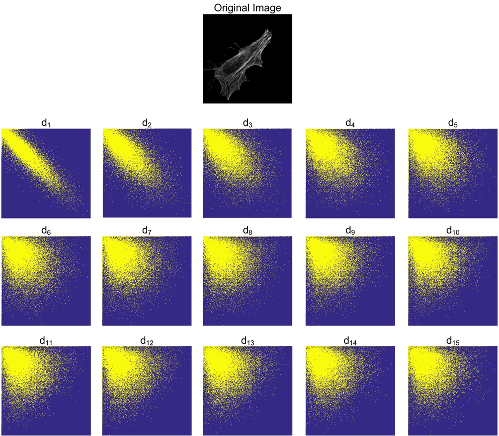

Close

Figure 3

GLCMs are constructed with varying values of parameter d for protein “original image” at the top.

Export to PPT

Consequently, the extracted features from these GLCM matrices possess diversified information related to textural appearance of images. The size of GLCM is dependent upon the gray level values held by an image and not on the image size itself. Let I be an image with N gray levels, the GLCM for image I will be an N-by-N dimensional matrix. This GLCM, at location (i, j), records the number of times two intensity levels i and j co-occur in the image I at distance d from each other at orientation θ. GLCM, of an image I with r rows, c columns and offset (d_x, d_y), can be represented mathematically as given in Eq. (1).

However, the GLCM is required to hold the probability rather than the count of the co-occurrence of any two intensities. Therefore, the GLCM entries are transformed so that they indicate probabilities. For this purpose, the number of times a particular combination of intensities occurs is divided by the total number of possible outcomes, in order to obtain probabilities. These probabilities are not true probabilities rather these are approximations. True probabilities require continuous values whereas the entries of GLCM are discrete values. Eq. (2) is used to transform a GLCM into approximate probabilities.

Here i and j represent the row and column of a GLCM, $V(i\text{,}j)$ indicates the total number of co-occurrences of intensity levels i and j whereas the summation in the denominator is the total number of co-occurrences of (i, j) (Do-Hong et al., 2010; Haralick, 1979).

One important issue related to GLCM is its size, which depends upon the gray levels of an image. For different combinations of (d, θ), there are four different possible GLCM matrices. Images, with a large number of gray levels, produce GLCM matrices that have huge amount of data storage requirements. Therefore, images are usually quantized to a low number of gray levels. However, reducing gray levels in an image may result in loss of texture information. Further, with a low number of gray levels homogeneity is more likely in such images (Chaddad et al., 2011; Liang and Malm, 2012). On the other hand, a large number of gray levels possess more detailed information for discrimination among patterns. However, this results in GLCM matrices, which are more sparse in nature and likely to have large vacancy level.

In this connection, we explore the effect of various quantization levels in conjunction with different values of offset parameter d on the information capturing capability of GLCM for fluorescence microscopy protein images. Distinct quantization levels as well as different values of offset parameter d result in different GLCM matrices and therefore, their produced feature spaces are diverse in nature. The occupancy level of GLCM is also affected by smooth image regions. For homogeneous images, the resultant GLCM will have higher count for some indices and most of the entries will correspond to zero. In such cases, the constructed GLCM should be based on distant neighbors (Srinivasan and Shobha, 2008). Therefore, using larger values of offset parameter d in constructing GLCMs for such images will help in extracting more information.

2.4 Haralick texture features

Haralick (Haralick, 1979) proposed the extraction of 14 statistical measures from a GLCM, which can better discriminate the texture. These features found many applications related to texture analysis and pattern classification (Hamilton et al., 2006; Haralick, 1979; Nanni et al., 2010c; Rathore et al., 2014). In this work, we utilized 13 of them including inertia, entropy, energy, correlation, inverse difference moment, sum variance, sum average, sum entropy, difference variance, difference average, difference entropy and two information measures of correlation. As discussed in Section 2.2, feature spaces from GLCM_V are averaged with GLCM_H and GLCM_D with GLCM_oD. The resultant averaged feature spaces are then concatenated with each other to produce 26-D feature space for each protein image.

2.5 The hybrid model

In order to develop efficient classification systems, sometimes different individual feature spaces are combined to collectively utilize their discriminative power. In this study, a number of hybrid models have been developed by concatenating different feature spaces. The detail is given as under:

• ${\mathbf{Har}}_{24}^{1''–''5}$ is composed of $\left\{{\text{Har}}_{24}^1\text{,}{\text{Har}}_{24}^2\text{,}{\text{Har}}_{24}^3\text{,}{\text{Har}}_{24}^4\text{,}\right.\left.{\text{Har}}_{24}^5\right\}$ producing 130-D feature space.

• ${\mathbf{Har}}_{24}^{6''–''10}$ is composed of $\left\{{\text{Har}}_{24}^6\text{,}{\text{Har}}_{24}^7\text{,}{\text{Har}}_{24}^8\text{,}{\text{Har}}_{24}^9\text{,}\right.\left.{\text{Har}}_{24}^{10}\right\}$ . This also produces feature space of 130-D.

• ${\mathbf{Har}}_{24}^{11''–''15}$ is composed of $\left\{{\text{Har}}_{24}^{11}\text{,}{\text{Har}}_{24}^{12}\text{,}{\text{Har}}_{24}^{13}\text{,}{\text{Har}}_{24}^{14}\text{,}\right.\left.{\text{Har}}_{24}^{15}\right\}$ . Here the output feature space dimension is also 130-D.

• ${\mathbf{Har}}_{24}^{1''–''15}$ is yielded by the concatenation of ${\text{Har}}_{24}^{1''–''5}\text{,}{\text{Har}}_{24}^{6''–''10}\text{,}{\text{Har}}_{24}^{11''–''15}$ . Here 390-D feature space is produced, since this hybrid model is the combination of all the 15 feature spaces for 24 gray levels in the original image.

Such models are developed for all the three datasets.

2.6 Correlation-based Feature Selection

In machine learning, feature selection is a preprocessing technique usually applied on data to select the most informative and discriminative features from the full feature space. In this way, redundant and irrelevant information is removed.

In this paper, we adopted CFS feature selection technique that is developed using the concept of filter based feature selection strategy (Hall and Smith, 1999). The concept behind the development of CFS is that selected features have high correlation with the target class whereas less correlation with each other. CFS utilizes the forward best first search strategy to search the useful features from the full feature space by starting with the empty set. It stops its operations when five consecutive subsets with no improvements are produced.

In this paper, we applied CFS on the ${\text{Har}}_{24}^{1''–''15}$ hybrid model for all the three datasets on the intention that first combine the discriminative power of all the feature spaces and then enhance this power by removing the redundant information. In this connection, from 390-D full feature space, CFS produced 33-D selected feature space for HeLa dataset, 40-D selected feature space for CHO dataset, and 31-D selected feature space for LOCATE Endogenous dataset.

2.7 Classification and ensemble generation

SVM is a well known and efficient classifier utilized by many researchers for addressing various problems in different application domains (Rathore et al., 2015; Rehman et al., 2013). In the current work, SVM with RBF kernel is trained using ${\text{Har}}_g^d$ for d = 1, 2, 3, …, 15 and g = 4, 8, 12, 16, 20, and 24. These classifications will be referred to as ${\text{SVM}}_g^d$ in this text where ${\text{SVM}}_g^d$ is trained using ${\text{Har}}_g^d$ feature space.

The individual classifications using all the feature spaces are recorded. In order to enhance the prediction performance of the proposed prediction system further, the individual classification results have been combined using Eq. (3).

The final output is obtained through the integration of individual prediction results using the majority voting scheme as given in Eq. (5).

Ensembles are built corresponding to all the offset values of every gray level quantization. The best ensemble is selected for building the final model of GLCM-SubLoc protein classification system.

3.1 Performance analysis of GLCM-SubLoc for HeLa dataset

The performance accuracies of the proposed GLCM-SubLoc prediction system are shown in Table 1. The first column indicates the value of the parameter d, which is the distance between the pixels to be checked for co-occurrence in constructing GLCM. The rest of the columns show the accuracy values yielded by GLCM-SubLoc utilizing the features from ${\mathit{GLCM}}_g^d$ for different d and g values.

It is observed that using the same gray level for different values of distance d varying from 1 to 15, there is very little variation in the accuracy values. The best values are obtained for d = 1 in all cases except for the gray level value of 24 where the best value of accuracy is yielded for d = 14. On the other hand, gradual enhancement in the accuracy values for the same value of d with varying gray levels is observed. The difference is initially higher, however, for gray levels 16, 20 and 24, this difference is small.

Almost same performance by the prediction system for different values of d shows that the patterns and information present in HeLa protein images is identical. The co-occurrence distribution of different intensities over the protein image is leading the classifier to show the same performance. However, when more information is added to the GLCM by varying the gray levels, the prediction performance of proposed model is enhanced. For the gray levels 20 and 24, the prediction performance has not been improved due to the redundancy in the information preserved by the two GLCMs from which the features are extracted.

Supplementary Table 1 demonstrates the detailed results for HeLa dataset. The performance of the proposed prediction system is demonstrated through sensitivity, specificity, MCC and F-score for different gray levels and for different values of GLCM offset parameter. Quite good performance is revealed from the quantitative analysis of the presented prediction values. The performance measures validate the good performance of the proposed prediction system.

The performance of the proposed prediction system using different hybrid models is shown in Table 2. The hybrid models have shown improved performance in some cases whereas comparable performance in some other.

The ${\mathbf{Har}}_{24}^{1-5}$ hybrid model has shown 5.6% improvement over the individual features for gray level value g = 24 and d values 1–5 where the highest accuracy in the range from 1 to 5 in Table 1 is 80.9%. However, ${\mathbf{Har}}_{24}^{6-10}$ hybrid model has shown low accuracy compared to the accuracies in the range of 6–10 for d values against gray level value g = 24 where the highest accuracy in this range is 81.0%. Similarly, the performance of ${\mathbf{Har}}_{24}^{11''–''15}$ hybrid model is lower than the individual accuracies in the range 11–15 for different d values for the same gray level value. On the other hand, the performance of the proposed prediction system using ${\mathbf{Har}}_{24}^{1''–''15}$ hybrid model is 88.2%, which is 6.9% higher than the highest accuracy in the range 1–15 for different d values. This reveals that the hybrid model has enhanced the prediction performance of the proposed prediction system compared to the individual feature spaces. The performance of the proposed prediction system using the CFS based selected feature space has shown comparable performance that is 88.3% compared to the ${\mathbf{Har}}_{24}^{1''–''15}$ hybrid model. However, the dimensionality of the CFS based features is 33-D compared to the 390-D dimensionality of the full feature space. The results obtained through the majority voting scheme for HeLa dataset are presented in Table 3. For each gray level value under consideration there are GLCMs for different values of offset parameter d ranging from 1 to 15 as discussed earlier. Ensemble is constructed from the results of 15 classifications for the same gray level. For example, taking into account GLCM of 4 gray levels, there are 15 values for the parameter d hence producing 15 classifications. In order to form an ensemble, the 15 classifications for the GLCM of 4 gray levels are employed.

The highest ensemble accuracy is reported for the ensemble constructed for the gray levels 16 and 24. However, the similarity measure Q-statistic shows low similarity among the members of the ensemble using GLCMs of 16 gray levels. This indicates that GLCMs of 16 gray levels produce informative and discriminative features for the classification stage. Fig. 4 shows the comparison among the ${\mathbf{Har}}_{24}^{1''–''5}$ , ${\mathbf{Har}}_{24}^{6''–''10}$ , ${\mathbf{Har}}_{24}^{11''–''15}$ , ${\mathbf{Har}}_{24}^{1''–''15}$ , the CFS based selected feature space, and the results of the majority voting based ensemble.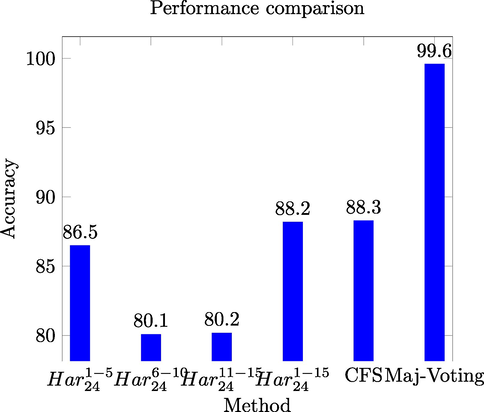

Close

Figure 4

Performance comparison for different models of HeLa dataset.

Export to PPT

The highest performance among different approaches for HeLa dataset is achieved through the majority voting scheme, which is yielded by integrating the decisions of different support vector machines.

3.2 Performance analysis of GLCM-SubLoc prediction system for CHO dataset

Performance assessments of the proposed prediction system for CHO dataset are presented in Table 4. The first column shows different values for the GLCM offset parameter d whereas the rest of the columns show accuracy values for the ${\text{Har}}_g^d$ features extracted from ${\text{GLCM}}_g^d$ .

It is observed that for a certain gray level, the accuracy value keeps increasing for the higher value of GLCM offset parameter d. This indicates that the co-occurring intensity values at larger distances possess more discriminative information compared to smaller values of d for this particular dataset. That is why the discriminative power of the classification system is enhanced with larger distances. Similarly, for a certain value of the distance parameter d, higher accuracies are achieved while utilizing features from GLCMs with more gray levels. In these results, GLCMs with gray level value of 16 might be enough for feature extraction.

This shows that prior to the development of a prediction model for classification, protein images coming from a particular source should be analyzed first for their patterns. Here, it is observed that higher accuracies are achieved for CHO dataset when the value of GLCM distance parameter d is 8 or above for all the gray levels presented in Table 4. Detailed results for CHO dataset are shown in Supplementary Table 2 where the performance achieved is demonstrated in terms of sensitivity, specificity, MCC and F-score. The assessments shown with different measures validate the performance of the proposed prediction model.

Hybrid models, utilized by the proposed prediction system, have shown improvement over the individual feature spaces as shown in Table 5. ${\text{Har}}_{24}^{1''–''15}$ achieved 1.4% higher accuracy compared to the highest accuracy achieved by the same features for d = 15 and g = 24 as shown in Table 4.

However, CFS based feature selection has also shown comparable performance against the hybrid models. This shows that feature selection or hybridization is unable to improve the performance of the prediction system. However, CFS based feature selection has reduced the dimensionality of the feature space from 390-D to 40-D only. On the other hand, the majority voting based ensemble outperformed all the adopted approaches in predicting protein localization from CHO dataset.

Table 6 presents the ensemble performance for CHO dataset. The first row shows the ensemble accuracy whereas the second row indicates the value for Q-statistic.

The highest ensemble accuracy is reported for the GLCMs of 12 and 16 gray levels where the accuracy value is 100% in both cases. The Q-statistic value shows the highest diversity for the members of these two ensembles. The GLCMs of gray level 12 and 16 for different values of distance parameter d produce feature spaces with diversified information, hence producing classifications of higher diversities. This leads to the higher performance of the ensemble classifier.

Fig. 5 shows the comparison among the ${\mathbf{Har}}_{24}^{1''–''5}$ , ${\mathbf{Har}}_{24}^{6''–''10}$ , ${\mathbf{Har}}_{24}^{11''–''15}$ , ${\mathbf{Har}}_{24}^{1''–''15}$ , the CFS based selected feature space, and the results of the majority voting based ensemble.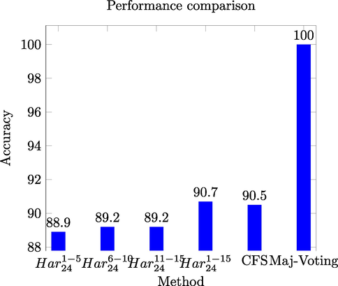

Close

Figure 5

Performance comparison for different models of CHO dataset.

Export to PPT

It is evident from Fig. 5 that majority voting based ensemble has shown significant performance in classifying protein images from fluorescence microscopy images of CHO dataset.

3.3 Performance analysis of GLCM-SubLoc prediction system for LOCATE Endogenous dataset

Performance accuracies of the proposed GLCM-SubLoc prediction system are presented in Table 7 for LOCATE Endogenous dataset. The first column shows different values of distance parameter d for GLCM construction whereas the remaining columns show the accuracy values achieved using features extracted from GLCM with different gray levels varying from 4 to 24.

The results presented show that there is some improvement in the classification accuracy for smaller values of d. For example, performance is better using the ${\text{Har}}_4^3$ , ${\text{Har}}_{12}^3$ , and ${\text{Har}}_{16}^3$ features from ${\text{GLCM}}_4^3$ , ${\text{GLCM}}_{12}^3$ , and ${\text{GLCM}}_{16}^3$ , respectively. The highest accuracy values using gray level values of 4, 12, and 16 with d = 3 are 82.0%, 88.4%, and 89.2%, respectively. Further increasing the value of d for a certain gray level did not enhance the performance. This shows that for LOCATE Endogenous dataset, a reasonable value of d might be between 2 and 8 inclusive. For other values, the performance is usually observed to be degraded.

As far as gray levels are concerned, 16 gray levels are sufficient to generate informative features from respective GLCMs for protein images of LOCATE Endogenous dataset as can be observed from the results shown in Table 7.

The detailed performance predictions are provided in Supplementary Table 3, which demonstrates the performance of the prediction system in terms of sensitivity, specificity, MCC and F-score. The performance predictions show that the proposed prediction system has efficiently classified the protein images from LOCATE Endogenous dataset into different classes.

The hybrid models for LOCATE Endogenous dataset, as shown in Table 8, have shown improvement over individual feature spaces. The highest performance accuracy 92.6% is achieved by the proposed prediction system using ${\text{Har}}_{24}^{1''–''15}$ hybrid model. This signifies the collective discrimination power of all the individual feature spaces.

Similarly, the CFS based selected feature space has shown slight improvement over ${\text{Har}}_{24}^{1''–''15}$ hybrid model, which is good achievement as far as dimensionality of the feature space is concerned. The CFS based feature space dimensionality is only 31-D achieving 92.2% accuracy as compared to the 390-D dimensionality of the full feature space achieving 92.6% accuracy.

The ensemble performance for LOCATE Endogenous dataset is shown in Table 9. The highest ensemble accuracies are recorded for GLCMs of 8, 20 and 24 gray levels. However, the highest diversity is achieved for the members of ensemble at gray levels 24 as shown by the Q-statistic value of 0.14.

This indicates that for this particular dataset, GLCMs might be constructed with either 8, 20 or 24 gray levels. The comparison among ${\text{Har}}_{24}^{1''–''5}$ , ${\text{Har}}_{24}^{6''–''10}$ , ${\text{Har}}_{24}^{11''–''15}$ , ${\text{Har}}_{24}^{1''–''15}$ , the CFS based selected feature space, and the results of the majority voting based ensemble is shown in Fig. 6.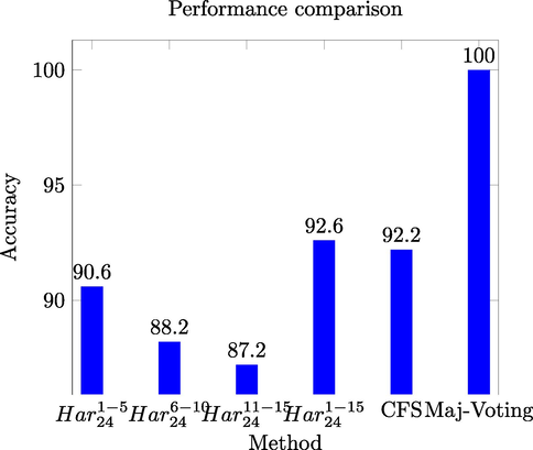

Close

Figure 6

Performance comparison for different models of LOCATE Endogenous dataset.

Export to PPT

The performance comparison for LOCATE Endogenous dataset reveals that majority voting based ensemble outperformed other approaches.

References

- Molecular Biology of the Cell (fourth ed.). National Center for Biotechnology Information∼Os Bookshelf; 2002.
- Automated recognition of patterns characteristic of subcellular structures in fluorescence microscopy images. Cytometry. 1998;33:366-375.
- [Google Scholar]
- A neural network classifier capable of recognizing the patterns of all major subcellular structures in fluorescence microscope images of HeLa cells. Bioinformatics. 2001;17:1213-1223.
- Improving of colon cancer cells detection based on Haralick’s features on segmented histopathological images. In: IEEE International Conference on Computer Applications and Industrial Electronics (ICCAIE), 2011. Penang: IEEE; 2011. p. :87-90.
- A multiresolution approach to automated classification of protein subcellular location images. BMC Bioinf.. 2007;8:210.
- Scene classification based on gray level-gradient co-occurrence matrix in the neighborhood of interest points. In: IEEE International Conference on Intelligent Computing and Intelligent Systems, 2009. ICIS 2009. Shanghai: IEEE; 2009. p. :482-485.
- Automated interpretation of subcellular patterns in fluorescence microscope images for location proteomics. Cytom. Part A J. Int. Soc. Adv. Cytom.. 2006;69A:631-640.
- Predicting membrane protein types by incorporating protein topology, domains, signal peptides, and physicochemical properties into the general form of Chou’s pseudo amino acid composition. J. Theor. Biol.. 2013;318:1-12.
- Cooper, G.M., 2000. The Cell: A Molecular Approach, second ed. ASM Press, Sunderland, Mass.: Sinauer Associates, Washington, D.C.
- A new descriptor for image retrieval using contourlet co-occurrence. In: Third International Conference on Communications and Electronics (ICCE), 2010. Nha Trang: IEEE; 2010. p. :169-174.
- Increasing the discrimination power of the co-occurrence matrix-based features. Pattern Recognit.. 2007;40:2367-2372.
- Automated subcellular location determination and high-throughput microscopy. Dev. Cell. 2007;12:7-16.
- Feature Selection for Machine Learning: Comparing a Correlation-Based Filter Approach to the Wrapper. In: Proceedings of the Twelfth International Florida Artificial Intelligence Research Society Conference. Orlando, Florida: AAAI Press; 1999. p. :235-239.
- Hamilton, N.A., Pantelic, R.S., Hanson, K., Fink, J.L., Karunaratne, S., Teasdale, R.D., 2006. Automated subcellular phenotype classification: an introduction and recent results. 2006 Work. Intell. Syst. Bioinforma. (WISB 2006).
- Protein subcellular location pattern classification in cellular images using latent discriminative models. Bioinformatics. 2012;28:i32-i39.
- 3D Co-occurrence Matrix Based Texture Analysis Applied to Cervical Cancer Screening. Uppsala, Sweden: Dep. Inf. Technol. Uppsala University; 2012.
- Boosting multiclass learning with repeating codes and weak detectors for protein subcellular localization. Bioinformatics. 2007;23:3374-3381.
- Abdominal tumor characterization and recognition using superior-order cooccurrence matrices, based on ultrasound images. Comput. Math. Methods Med.. 2012;2012:17.
- Robust numerical features for description and classification of subcellular location patterns in fluorescence microscope images. J. VLSI Signal Process.. 2003;35:311-321.
- Different approaches for extracting information from the co-occurrence matrix. PLoS One. 2013;8:e83554.
- Novel features for automated cell phenotype image classification. Adv. Comput. Biol. Adv. Exp. Med. Biol.. 2010;680:207-213.
- Selecting the best performing rotation invariant patterns in local binary/ternary patterns. Proc. Int. Conf. Image Process. Comput. Vision Pattern Recognit. 2010
- Fusion of systems for automated cell phenotype image classification. Expert Syst. Appl.. 2010;37:1556-1562.
- Location proteomics: systematic determination of protein subcellular location. In: Maly I.V., ed. Systems Biology. Humana Press; 2009. p. :313-332.
- Novel structural descriptors for automated colon cancer detection and grading. Comput. Methods Programs Biomed.. 2015;121:92-108.
- Ensemble classification of colon biopsy images based on information rich hybrid features. Comput. Biol. Med.. 2014;47:76-92.
- Chapter four – Predicting G-protein-coupled receptors families using different physiochemical properties and pseudo amino acid composition. Methods Enzymol.. 2013;522:61-79.
- Adaptive multiresolution techniques for subcellular protein location classification. IEEE Int. Conf. Acoust. Speech Signal Process. 2006
- Statistical texture analysis. Proc. World Acad. Sci. Eng. Technol.. 2008;36:1264-1269.
- Protein subcellular localization in human and hamster cell lines: employing local ternary patterns of fluorescence microscopy images. J. Theor. Biol.. 2014;340:85-95.
- Protein subcellular localization of fuorescence imagery using spatial and transform domain features. Bioinformatics. 2012;28:91-97.
- [CrossRef] [Google Scholar]
- Subcellular localization using fluorescence imagery: utilizing ensemble classification with diverse feature extraction strategies and data balancing. Appl. Soft Comput.. 2013;13:4231-4243.
- An incremental approach to automated protein localisation. BMC Bioinf.. 2008;9:445.
- Genetic algorithm optimization of adaptive multi-scale GLCM features. Int. J. Pattern Recognit. Artif. Intell.. 2003;17:17-39.
Appendix A
Supplementary data
Supplementary data associated with this article can be found, in the online version, at https://doi.org/10.1016/j.jksus.2016.12.004.