

Translate this page into:
Ordination classification of relationship of vegetation and soil’s edaphic factors along the roadsides of Wahcantt, Pakistan
⁎Corresponding author at: Department of Environmental Sciences, Fatima Jinnah Women University, The Mall, Rawalpindi 46000 Pakistan. drsaeed@fjwu.edu.pk (Sheikh Saeed Ahmad)
-
Received: ,
Accepted: ,
This article was originally published by Elsevier and was migrated to Scientific Scholar after the change of Publisher.
Peer review under responsibility of King Saud University.
Abstract
Vegetation and soil had reciprocal interrelated effects over each other. For this purpose, a study was carried along roadsides of WahCantt to determine relationship between vegetation and soil’s edaphic factors using ordination classification. Herbaceous data was collected using Braun Blanquet approach which identified 18 species of 36 families with Cynodon dactylon as the most dominant species. Relationship between soil’s edaphic factors (Zn2+, Cu2+, Fe2+, Mn2+, O.M, EC, pH) and species richness was determined using CCA. The dominant species of Cynodon dactylon was found to be only affected by EC. T-value biplots were employed to identify the response of herbaceous species against selected soil’s edaphic factors and Partial ordination for variation portioning of species against every edaphic factor. CCA had highlighted Zn2+ as the most influencing factor over the species distribution while Mn and O.M had no impact over species richness. T-value biplot of Fe2+ was found to be positively affecting the abundant species of Cynodon dactylon whereas no species had recorded its response against Mn and O.M. Cynodon dactylon was emerged to be least emerged species in bivariate scatter plots of partial ordination. The study highlighted the interrelationship between soil’s edaphic factor and herbaceous flora which would be helpful in determining limiting constraint in species distribution.
Keywords
CCA
T-value bi-plots
Partial ordination
Species distribution
Ordination classification

1 Introduction
Roads provide the easiest means of communication among the people living in different parts of world. Roads are important as they help in boasting up the trade and economic position of country by connecting it with different cities for competing with the International positions (Harper, 2001). Road verges help in supporting the habitat and for conservation of specie for maintaining nature’s value (Wilson et al., 1992) by acting as corridors, barriers or habitats for the distribution of plants and animal species (Angold, 1997).
Soil and vegetation are interrelated and do exert certain reciprocal effects on each other; soil gives support to vegetation i.e. moisture, nutrients and anchorage to grow effectively whereas vegetation supports the soil by providing protective cover, preventing or reducing soil erosion and also by maintaining soil nutrients through litter accumulation and decay (Farrag, 2012). The plants growing along the roadside are useful for overcoming the noise and chemical pollution and can improve the scenic beauty of roadside surroundings (Ullmann and Heindl, 1989; Ahmad and Jabeen, 2009). Determination of variability of soils has been of interest to soil scientists and geographers for quite long time. Information on soil properties is usually available from a limited number of point measurements and spatial estimates are prepared (Netler, 2001). Soil and vegetation relationship can be studied by multivariate or ordination techniques in which species are arranged along the gradients.
In some parts of world, mainly in Europe, North America and New Zealand, roadsides are given due importance for assessment of vegetation growing along with them (Sara, 2006). These roadsides provide habitat to plant species and sometimes to animals as well (Jesse et al., 2008) but sometimes developments of these roads may also result in habitat loss, pollution, native animal mortality and habitat fragmentation which lead to loss of biodiversity (Tromans, 1991; Spellerberg and Gaywood, 1993). Well organized legislative and infrastructure planning can overcome all these problems and help in providing habitat to animals, plants and can prevent from loss of biodiversity (Bennett, 1991; Brooks, 1993). Soil and roadside verges play considerable role in distribution of species in particular area thus constitute immense importance in ecology, urban planning, and economic growth thus providing conservational purpose for preventing habitat loss (Ahmad et al., 2013a,b).
Tsuyuzaki and Titus (2010) investigated the human impacts on roadside grassland vegetation of an Oak forest of Washington, USA by using CCA. For obtaining best results, vegetation and environmental data were collected for 48 plots with each plot cover consisting of 1 to 8 species having most of exotic species. Environmental variables including slope, tree canopy area, barren area, litter thickness and distance from the road were studied for finding the vegetation pattern. The result obtained from CCA showed that forest canopy area played an important role in forest development while litter thickness and soil firmness also affected the vegetation pattern. Distance from the road also affected the vegetation pattern but not affected as a primary factor. The study helped in predicting the specie richness, abundant exotic species and in the management and conservation of canopy cover for nature’s preservation.
Climate change has resulted in significant changes. Climate change has significantly affected the vegetation flora of Pothawar region of Pakistan. Change in vegetation was found in reported by Bashir and Ahmad (2017) as well as Butt et al. (2015). Significant urbanization is also reported in the aforementioned studies in respective area. Further, a study investigated the temperature variations and its impact over current vegetation along with other soil parameters (Gulshad et al., 2016).
The rationale behind this study is to quantify the vegetation along roadsides of Wah Cantt, to find out how different parameters of soil effect the distribution of vegetation and to study the soil vegetation relationship using ordination techniques across Wah Cantt Rawalpindi, Pakistan.
2 Materials & method
2.1 Study area
Wah Cantonment (Wah Cantt) is a military Cantonment located in the Punjab province near Taxila and in northwest of Islamabad (Pakistan’s capital city). Small valley of almost 58.27 km2 is surrounded by hills. Area is suitable for all types of vegetation. Geologically limestone, sand stone and alluvial deposits are found in this area. The study was carried out along the roadside verges of Wah Cantonment to analyze the relationship between soil and herbaceous flora. Wah Cantt lies between 33.7714° North latitudes and 72.7518° East longitudes. Wah Cantt is a military city located in the Punjab province of Pakistan, 30 km (19 mi) to the north west of Rawalpindi/Islamabad. The area of the city is 90.65 km2 (35.00 sq mile) and elevation is 471 m (1545 ft) (Bashir et al., 2016).
2.2 Herbaceous data
Field trips had been made for the collection of wild plant species in the month of April (in the spring season when the herbaceous plants were full on bloom). Studying plant cover in any areas required different approaches e.g. line transect and random walking sampling. In the present study, quadrat method was applied for vegetation classification, analysis and studying the relationship with environmental gradients. A 1 m long tape was laid down to mark the quadrat of 1 × 1 square meters. Only the herbaceous data was collected by a technique called Braun-Blanquet approach. The technique was used for the collection of ground flora through random sampling. Total 50 quadrats were laid down. The cover value was calculated through visual estimation, the method called Domin cover scale (Ahmad et al., 2013a,b). The vegetation data is collected 1–2 m away from both sides of roads because the green belts around the roads only contain fences and ornamental flowers.
2.3 Environmental data
Total 50 soil samples were collected and sent to the soil fertility survey and testing laboratory, Rawalpindi for tests. Soil was collected from the area of Wah Cantt with any unusual feature like dumping of waste, grazing, change in color, fire outbreak, water out flow and digging. Soil sampling is started from 1–15 cm in depth. Wooden and steel spatula (Khurpa) was used for digging and polythene bags were used for storage of soil that were marked with codes. 250 gm of soil was collected in each polythene bag. Samples were sent to laboratory for testing of Electrical conductivity, pH, Organic matter and micronutrients i.e. Zinc (Zn2+), Copper (Cu2+), Manganese (Mn2+) and Iron (Fe2+) (Table 1).
EC
pH
O.M%
Zn mg kg−1
Fe mg kg−1
Cu mg kg−1
Mn mg kg−1
Sample01
0.98
7.91
0.78
1.16
4.6
0.18
1.86
Sample02
0.92
7.85
0.67
1.1
4.41
0.16
1
Sample03
0.81
7.88
0.71
1.08
4.33
0.15
1.8
Sample04
0.78
7.89
0.7
1.04
4.21
0.11
1.76
Sample05
0.54
7.89
0.73
1.02
4.02
0.15
1.91
Sample06
0.32
7.91
0.77
1.06
4.38
0.23
1.67
Sample07
0.87
7.93
0.83
1.16
4.61
0.27
1.82
Sample08
0.92
7.85
0.59
0.86
4.21
0.22
1.17
Sample09
0.86
7.88
0.62
0.86
4.44
0.11
1.8
Sample10
1.01
7.86
0.57
0.92
4.3
0.16
1.76
Sample11
0.96
7.84
0.66
0.88
4.86
0.24
1.73
Sample12
0.91
7.87
0.54
0.73
4.12
0.2
1.62
Sample13
0.94
7.83
0.63
1.17
4.34
0.23
1.5
Sample14
0.89
7.93
0.71
1.13
3.98
0.21
1.43
Sample15
1.01
7.85
0.76
1.05
3.99
0.18
1.77
Sample16
0.78
7.87
0.69
1.01
4.67
0.22
1.89
Sample17
1.02
7.88
0.74
0.71
4.51
0.24
1.42
Sample18
1.09
7.89
0.78
0.91
4.9
0.26
1.56
Sample19
0.94
7.91
0.73
0.98
4.18
0.29
1.48
Sample20
1.07
7.82
0.77
0.84
3.87
0.21
1.43
Sample21
0.91
7.84
0.68
0.88
4.71
0.28
1.55
Sample22
0.89
7.81
0.85
0.98
4.33
0.18
1.84
Sample23
1.06
7.86
0.78
1.16
4.6
0.17
1.45
Sample24
1.05
7.91
0.57
1.08
4.55
0.21
1.9
Sample25
0.92
7.95
0.79
0.86
4.65
0.27
1.23
Sample26
1.04
7.86
0.77
1.14
4.87
0.24
1.7
Sample27
0.97
7.8
0.68
1.09
4.89
0.23
1.6
Sample28
0.56
7.88
0.65
1.17
4.8
0.19
1.5
Sample29
1.03
7.81
0.69
1.11
4.66
0.16
1.8
Sample30
0.67
7.89
0.7
1.04
3.94
0.24
1
Sample31
0.96
7.82
0.73
0.87
4.54
0.27
1.9
Sample32
0.56
7.91
0.77
0.67
3.9
0.24
1.1
Sample33
1.08
7.87
0.78
0.95
4.43
0.28
1.86
Sample34
1.03
7.82
0.85
0.84
4.67
0.13
1.93
Sample35
1.07
7.92
0.74
0.87
4.44
0.23
1.84
Sample36
1.25
7.85
0.8
0.86
4.82
0.11
1.81
Sample37
1.09
7.8
0.83
0.99
4.9
0.16
1.72
Sample38
1.08
7.86
0.79
0.98
4.76
0.26
1
Sample39
1.07
7.91
0.62
0.89
4.56
0.24
1.56
Sample40
1.4
7.81
0.71
0.98
4.57
0.18
1.74
Sample41
1.04
7.94
0.75
0.87
4.18
0.28
1.88
Sample42
1.09
7.84
0.78
0.89
4.88
0.19
1.81
Sample43
1.04
7.88
0.83
0.9
4.6
0.15
1.23
Sample44
1.05
7.82
0.73
0.91
4.82
0.29
1.66
Sample45
1.07
7.92
0.66
0.94
4.71
0.18
1.24
Sample46
1
7.6
0.68
0.98
3.98
0.19
1.39
Sample47
1.03
7.88
0.83
1.16
3.91
0.25
1.45
Sample48
0.92
7.83
0.79
1.17
4.66
0.18
1.47
Sample49
0.89
7.9
0.65
0.86
4.6
0.16
1.88
Sample50
0.96
7.87
0.67
1.04
3.9
0.18
1.5
2.4 Ordination classification
CCA was utilized for finding the relationship of floristic data with selected environmental variables. CANOCO 4.5 software was used for carrying out CCA. The sub techniques of CCA employed were t-value bi-plot and Partial ordination. T-value bi-plot, was employed for verifying response of species association (whether positive or negative) against any environmental variables while partial ordination was employed to illustrate different classes of data for ensuring their abundance against environmental parameters.
3 Results
3.1 CCA
The edaphic factors that were selected to find the relationship between environmental variables and species were electrical conductivity, pH, organic matter, zinc, copper, iron and manganese. The blue colored triangle in graph represents the species while the red color arrows represent selected environmental variables. The environmental variables with long arrow head had more impact on plant community and species distribution. The angle between an arrow and each axis represents the degree of correlation with that axis (Bruelheide and Udelhoven, 2005). The species that were closest or nearer to the arrow were strongly affected by the edaphic factor and the species that were far away were less influenced. The distance between the points reflects the degree of association between different species within same quadrat. If in a particular quadrat, at the same point, multiple species were present than it means that they had same abundance value and influenced by particular factor in same way (Braak and Looman, 1994). The arrow of Zinc was longest than any other variable of CCA bi-plot. Zinc has strongly affected the specie of Cucumis meloagrestis while the other species nearer or closest to the arrow head of Zn are positively influenced. The presence of Organic matter and Manganese had no impact upon the presence or absence of any species. The arrow heads of pH had an impact on Euphorbia hirta and nearest species to the arrow head of pH were positively influenced. The environmental gradient EC had remarkable effect on the specie of Sisymbrium irio, Oxalis corniculata, Rumex dentatus and Capsella bursa patoris. Copper only influenced the specie of Cynodon dactylon while iron impacted the Lycopericon esculentum (Fig. 1).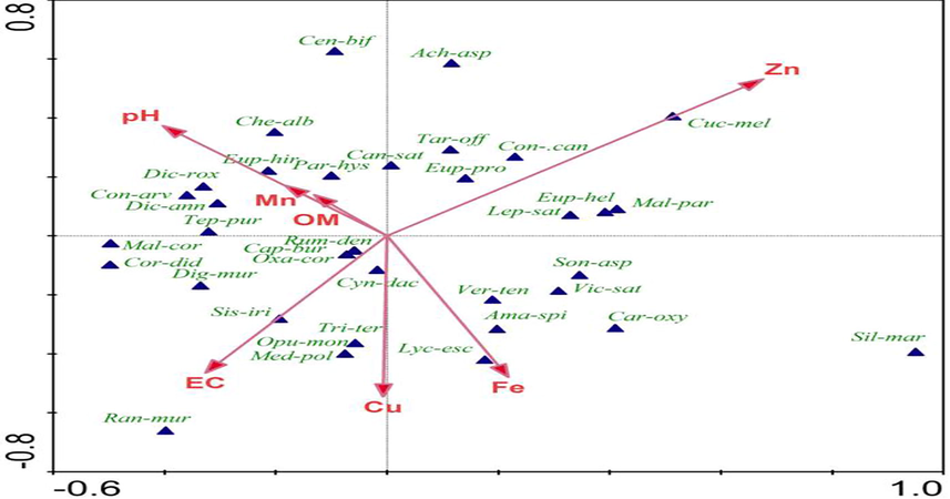
CCA bi-plot for species and environmental variables.
A study was carried out along the roadside of Havalian city in CCA was applied as a multivariate technique along with DCA. To check the relationship of vegetation and soil, EC and pH were used as environmental variables. The results obtained from the study revealed that species had strong relation with soil temperature and EC showing that EC and temperature were playing a role in determining the abundance/scarcity of species while pH had no significant impact on abundance or scattering of species (Ahmad et al., 2013a,b).
3.2 T-value biplots
The use of T-value bi-plot helps in inferring whether particular species reacted considerably to any particular environmental variable and if environmental variables reacted considerably to the regression of particular species (Leps and Smilauer, 2003). It could be applied for estimation of t-value regression coefficients, for multiple regression with specific species. Coordinates for species and environmental variables were plotted on same scale. The points for species indicated the critical value t-value 2. In order to find out the behavior of particular specie with particularly selected environmental gradient or variable, red circles were drawn for illuminating positive response in such a way that circle was drawn with its center midway between arrowhead for that variable and the origin of coordinate system. The total diameter of circle was equal to the length of that variable arrow. Specie line that had finished within the circle had positive regression coefficient with that variable and had t-value greater than 2. Similar circle was drawn in opposite direction with blue color for showing negative regression coefficients. These two circles which were drawn to illuminate the positive and negative regression coefficients were called Vann Dobben circles (Draper and Smith, 1981).
The t-value bi-plot of pH had shown that the arrowhead of Convolvulus arvensis was passing through red circle, means its growth was preferred in the presence of high pH as compared to others species arrow passing through the circle. The species Silybum marianum, Vicia sativa and Verbena tenuisecta had recorded negative response to the pH content which means presence of pH content played a role in suppressing their growth. The arrows of Euphorbia heliscopia and Ranunculus muricatus were also showing to be effected but the effect is insignificant. While the other species of Cucumis meloagrestis, Lepidium sativum, Taraxacum officinale, Oxalis Corniculata, Chenopodium album, Convolvulus arvensis and Achyranthes asper were remain unaffected to the pH content.
Species of Medicago polymorpha, Malvastrum coromandelianum, Convolvulus arvensis, Coronopus didymus, Capsella bursa patoris, Dicliptera roxburghiana and Rumex dentatus was passing through red circle but the species of Capsella bursa patoris, Dicliptera roxburghiana and Rumex dentatus had shown more positive response as they were nearer to the arrow head of circle which means that these species grow well or had elevated level of abundance in the presence of EC content while presence of EC had more negative impact on the species of Cucumis meloagrestis, Lepidium sativum and Taraxacum officinale as compared to Euphorbia heliscopia, Oxalis corniculata, Chenopodium album, Convolvulus arvensis and Achyranthes asper. Negative response of species was recorded by blue circles while the other species of Silybum marianum, Vicia sativa, Verbena tenuisecta and Ranunculus muricatus remained unaffected in the presence of EC while OM and Mn had shown no positive and negative response. In the T-value bi-plot of Zn, the arrow head of Euphorbia heliscopia is passing through the red circle which means it is showing positive response and its growth was enhanced in the presence of Zn as compare to other species while the species of Medicago polymorpha, Ranunculus muricatus and Malvastrum coromandelianum was showing negative response, means their growth was suppressed in the presence of Zn while the other species had shown insignificant response to the presence or absence of Zn. Cu was found to be positively effecting the species of Medicago polymorpha had shown the positive response to the presence of copper which means its growth is elevated in the presence of copper while insignificant negative response was recorded for species of Taraxacum officinale, Conyza canadensis, Cenchrus biflorus Roxb, Euphorbia prostrate, Cannabis sativa and Achyranthes asper .The species of Malvastrum coromandelianum, Oxalis corniculata, Tephrosia purpure, Lepidium sativum and Euphorbia heliscopia were remained totally impassive while Fe had positively affected the species of Medicago polymorpha and Cynodon dactylon was passing through red circle. So their behavior towards iron content was positive and significant. The abundance, growth and scattering of these species was high in presence of iron while iron content had slight negative effect on the specie of Malvastrum coromandelianum as it was passing through blue circle and had dependency for lower values of explanatory variables. While the species of Conyza canadensis, Ranunculus muricatus and Coronopus didymus were remain unaffected to iron content (Fig. 2).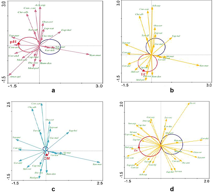
T-value bi-plots a. pH, b. EC, c. OM, d. Zn, e. Cu, f. Fe, g. Mn.
T-value bi-plots a. pH, b. EC, c. OM, d. Zn, e. Cu, f. Fe, g. Mn.
Ahmad et al. (2013a,b) used T-value biplot to determine the species richness in relation to particular environmental gradients i.e. soil pH and soil moisture in Changa manga forest. Species Rumex crispis, Sonchus oleoraceous, Prosopis cineraria, Desmostachya bipinnata, Cynodon dactylon, Malvastrum coromendialinum, Ageratum conyzoid, Sonchus arvensis and Conyza canadensis showed positive response towards soil moisture while the species holding negative response towards negative response circle were Conyza bonariensis, Mentha spicata, Parthenium hysterophorous, Suaeda fruiticosa, Prosopis cineraria, Chenopodium album, Ranunculas muricatus, Stelleria media and Taraxacum officinale.
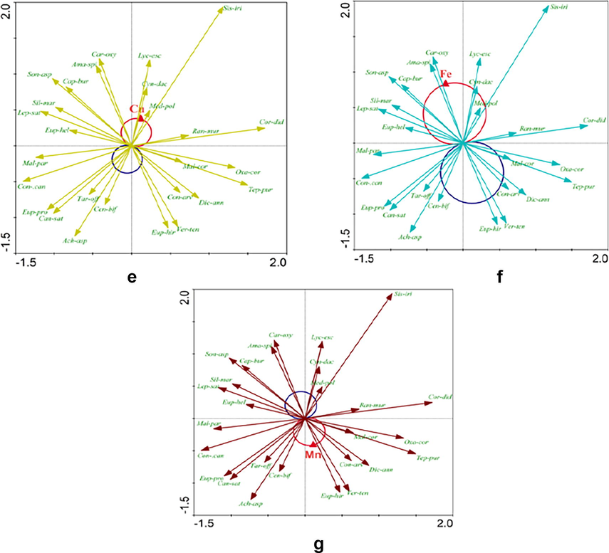
3.3 Partial ordination
Scatter plot is a visual representation of bivariate set which shows the relationship between the two variables and these two variables facilitate the regression model or correlation coefficient. The results of scatter plot were displayed in the form of Pie charts showing the selected environmental variables i.e. EC, pH, Organic matter, micro-nutrients containing Zinc, Copper, Iron and Manganese in each sample. Pie chart is a circular chart which represents the data quantitatively and each circle in it is divided into various parts or slices depending upon the presence of selected variable (Ahmad et al., 2013a,b).
The range of interval for EC is from 0.32 to 1.4 with average of 0.948 and median is 1.285. The selected class interval is 4 and as a result of it 4 classes were formed with Class-I contains13 members, class-II contains 12 members, class III contains 13 members & class IV contains 12 members. Interval of class-1 was from 0.32–0.89 and it contained the species of Achyranthes asper and Chenopodium album. Species of Ranunculus muricatus, Tribulus terrestris and Opuntia monacantha only existed in class of EC-2 and in the interval of 0.89–0.97. Malvastrum coromandelianum and Sonchus asper subsisted in the interval of 0.97–1.05 and showed its dominance in EC-3.
The range of interval for pH was from 7.6 to 7.95 with average of 7.869 and median 7.867. Total four classes were formed with class-I contains15 members, class-II contains 12 members class III contains 11 members while Class IV contains 12 members. Species of Ranunculus muricatus only existed in class of pH-1 and in the interval of 7.6–7.84. Malvastrum coromandelianum and Sonchus asper subsisted in the interval of 7.84–7.87 and showed its dominance in pH-2.The species of Achyranthes asper, Chenopodium album, Cenchrus biflorus Roxb and Sisymbrium irio appeared dominant for the interval of 7.87–7.9 in class of pH-3. While for O.M the range of interval was from 0.54 to 0.85 with average of 0.7226 and median 0.73. Total four classes were formed with class-I contains13members, class-II contains 14 members, class III contains 13 members and class IV contains 10 members. The dominating species of O.M-1 existed from interval of 0.54–0.67 and it had the species of Chenopodium album. The class of O.M-2 was recorded from 0.67–0.73 and for the species of Achyranthes asper, Ranunculus muricatus, Tribulus terrestris and Opuntia monacantha. The species of Sonchus asper and Sisymbrium irio appeared dominant for the interval of 0.73–0.78 in O.M-3.
The upper inclusive limit for Zn was 0.67–1.17. Median was 0.98 and average was 0.9786 and selected class interval was four and as a result of it total four classes were formed with class-I contains14members, class-II contains 13 members, class III contains 11 members while class IV contains 12 members. The species of Digera muricata, Tribulus terrestris and Opuntia monacantha appeared dominant in class of Zn-1, Zn-2 was dominated by Sisymbrium irio, Zn-3 by Achyranthes asper and Zn-4 by Sonchus asper and Malva parviflora. While the range of interval for Cu was from 0.11 to 0.29 with average of 0.2058 and median 0.21. Total four classes were formed with class-I contains13members, class-II contains 14 members, class III contains 13 members and class IV contains 10 members. The species of Achyranthes asper appeared dominant for the interval of 0.11–0.17 for class-1. Cu-2 was dominated by Digera muricata and Cu-3 by the species of Sonchus asper, Opuntia monacantha and Tribulus terrestris. The species of Carthamus oxyacantha appeared dominating for the interval of 0.24–0.29 in class-4.
The interval for Fe was from 3.87 to 4.9 with average of 4.4552 and median 4.454. Total four classes were formed having class-I contains14 members, class-II contains 11 members, class III contains 13 members and class IV contains 12 members. The dominating species of Fe-1 included Cenchrus biflorus Roxb, Opuntia monacantha and Tribulus terrestris for the interval of 3.87–4.21. Fe-2 appeared for the interval of 4.21–4.54 and was dominated by Achyranthes asper while Fe-3 was dominated by Digera muricata for the interval of 4.54–4.67. Fe-4 was dominated by Sonchus asper for the interval of 4.67–4.9. While the upper inclusive limit for Mn was 1–1.93. Median was 1.665 and average was 1.5984 and selected class interval was four and as a result of it total four classes were formed with class-I contains14 members, class-II contains 11 members, class III contains 13 members & class IV contains 12 members. The dominating species of Manganese-1 included Sisymbrium irio, Opuntia monacantha and Tribulus terrestris for the interval of 1–1.45. Manganese-2 appeared for the interval of 1.45–1.66 and was dominated by Amaranthus spinosus while Manganese-3 was dominated by Achyranthes asper and Sonchus asper. The class interval for Manganese-4 was from 1.81–1.93 and Digera muricata was the dominating species (Fig. 3).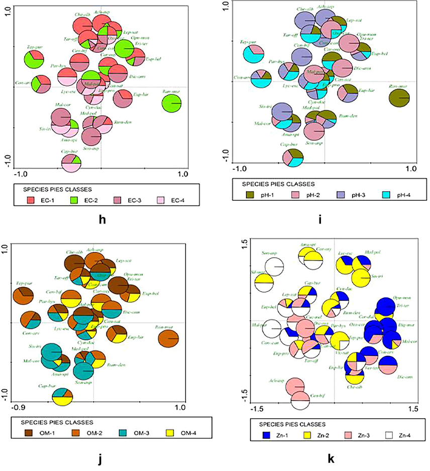
Partial ordination h. EC, i. pH, j. OM, k. Zn, l. Cu, m. Fe, n.
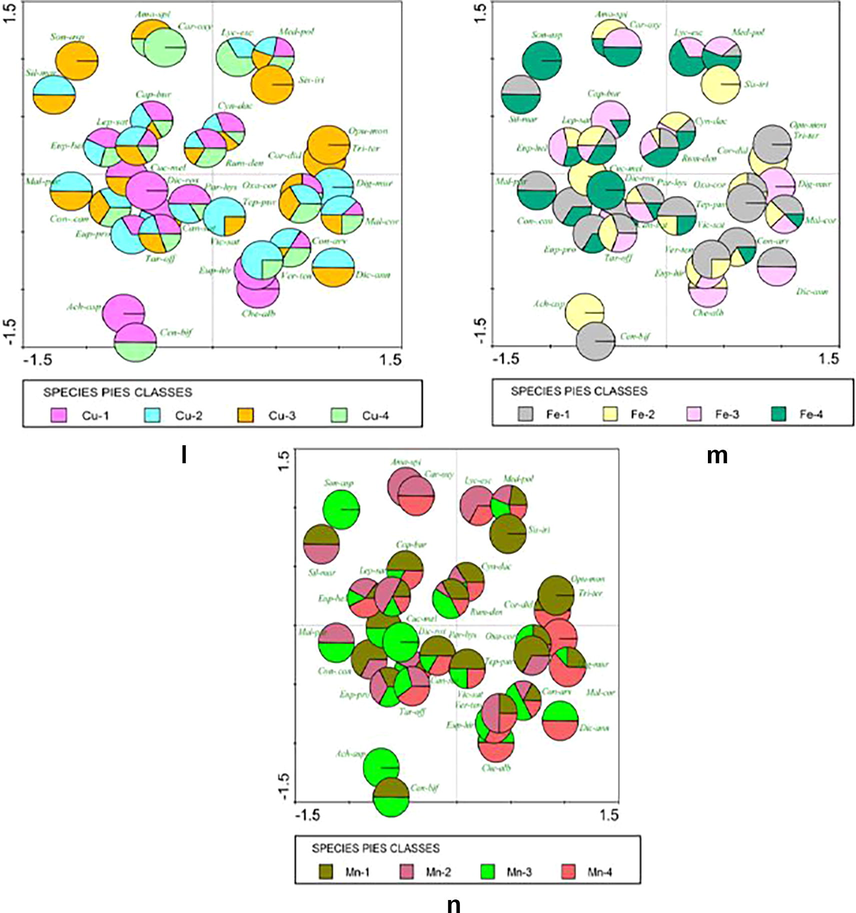
Partial ordination h. EC, i. pH, j. OM, k. Zn, l. Cu, m. Fe, n.
Ahmad et al. (2014) applied partial ordination in which moisture has 3 classes with species abundance in class 3. Ranunculus muricatus was abundant in EC while Cannabis sativa and Cynodon dactylon were lying in all four classes of pH and copper. Viciafaba and Veronica persica were abundant in EC while Melilotu sindica was abundant in phosphorus, iron and zinc. Veronica persica, Viciafaba and Ranunculus muricatus were abundant in potassium and manganese pie chart.
4 Conclusion
The world is facing the problem of climate change. This climate change greatly effects the floristic composition of any areas. The effect of climate change has left strong impact on the herbaceous flora of Wah Cantt. The species of “Tephrosia” is found to be growing in the area. Tephrosia is abundantly growing species of deserts and its presence indicates the changed climatic conditions of Wah Cantt. Riaz and Javaid (2009) indentified different species growing in Wah Cantt but Tephrosia was not present in 2009. Cannabis sativa appeared as the second most dominant weed. In 2009, Cannabis was reported as the most dominant species of Wah while Parthenium as the second most dominant species, but in 2014 the species of Cynodon appeared as the overruling species of Wah Cantt. The shift observed in the abundance of species might be due to the change in climatic conditions of an area. The study will be helpful in studying the native flora and in proper management of alien weeds growing in Wah Cantt.
5 Limitations of study
The conducted study has following limitations
-
The study itself doesn’t incorporated climatic evaluation but deduced results on the basis of already conducted studies in Potowar region.
-
The study investigated the particular locality and there was no data base available for cross checking the identified species or for its temporal analysis.
References
- Multivariate analysis of environmental and vegetation data of Ayub National Park Rawalpindi. Soil Environ.. 2009;28(2):106-112.
- [Google Scholar]
- Evaluating the effects of Soil pH and moisture on the plant species of changa Manga forest using Van Dobben Circles. Middle-East J. Sci. Res.. 2013;17(10):1405-1411.
- [Google Scholar]
- Exploring the general pattern of species distribution and abundances of changa manga forest correlating environment variables. World Appl. Sci.. 2013;28(8):1089-1092.
- [Google Scholar]
- Environmental diversification and Spatial variation in Riparian vegetation: a case study of Korang river, Islamabad Pakistan. Pak. J. Bot.. 2014;46(4):1203-1210.
- [Google Scholar]
- The impact of a road upon heathlands vegetation: effects in plants species composition. J. Appl. Ecol.. 1997;34:409-417.
- [Google Scholar]
- Exploring Geospatial techniques for spatio-temporal change detection in land cover dynamics along Soan River. Pakistan. Environ. Monit. Assess.. 2017;189:222.
- [Google Scholar]
- Multivariate Analysis for the assessment of herbaceous roadside vegetation of Wah Cantonment. J. Anim. Plant Sci.. 2016;26(2):457-464.
- [Google Scholar]
- Roads, roadsides and wildlife conservation: a review. In: Saunders D.A., Hobbs R.A., eds. Nature Conservation 2: The Role of Corridoors. Chipping Norton: Surrey Beatty and Sons; 1991. p. :99-118.
- [Google Scholar]
- Evaluation of Roadside Vegetation in central Arizona. University of Arizona; 1993. Ph.D. thesis
- Correspondence of fine scale spatial variation in soil chemistry and herb layer vegetation in beech forests. Forest Ecol. Manage.. 2005;210(3):205-223.
- [Google Scholar]
- Butt, A., Shabbir, R., Ahmad, S. S., Aziz, N., 2015. Land use change mapping and analysis using remote sensing and GIS: a case study of Simly watershed, Islamabad, Pakistan. E.J.R.S, vol. 18, pp. 251–259.
- Applied Regression Analysis. New York: Wiley; 1981.
- Floristic composition and vegetation-soil relationships in WadiAl-Argy of Taif region, Saudia Arabia. Int. Res. J. Plant Sci.. 2012;3(8):147-157.
- [Google Scholar]
- Differential responses of Vegetation along Effective Soil Gradients in Mughal Garden Wah Pakistan. Int. J. Econ. Environ. Geol.. 2016;7(1):36-41.
- [Google Scholar]
- Harper D., 2001. Horseboating (Web). The Horseboating Society. Retrieved on April 9, 2014.
- Road verges as invasion corridors? a spatial hierarchical test in an arid ecosystem. Landscape Ecol.. 2008;23(4):439-451.
- [Google Scholar]
- Multivariate analysis of Ecological data using CANOCO. New York: Cambridge University Press; 2003. p. :121-123.
- Volume modeling of soils using GRASS GIS 3D-Tools. Germany: Hannover; 2001.
- Invasion of hostile alien weed Parthenium Hysterophorus L. in Wah Cantt, Pakistan. J. Anim. Plant Sci.. 2009;19(1):26-29.
- [Google Scholar]
- Plant species richness in midfield islets and road verges-The effect of landscape fragmentation. Biol. Conserv.. 2006;127(40):500-509.
- [Google Scholar]
- Spellerberg, I.F., Gaywood, M.J.,1993. Linear Features: linear Habitats and wildlife corridors. English Nature. Research Report no. 60.
- Roadside grassland vegetation in an Oak forest, Oak Creek wildlife area, the Cascade Range USA. iForest. 2010;3:52-55.
- [Google Scholar]
- Geographical and ecological differentiation of roadside vegetation in temperate Europe. Bot. Acta. 1989;102:261-269.
- [Google Scholar]
- Distribution and some climatic correlations of some exotic species along roadsides in New Zealand. J. Biogeogr.. 1992;19:183-194.
- [Google Scholar]


