Optimizing structure-property models of three general graphical indices for thermodynamic properties of benzenoid hydrocarbons

Data availability

The data generated related to this study is available in a public repository on GitHub https://github.com/Sakander/Predictive_Potential_General_Indices.git.

1 Introduction

Cheminformatics employs quantitative structure–property relationship (QSPR) studies (Katritzky et al., 2001) in order to estimate various thermodynamical and physicochemical characteristics of molecular compounds especially, organic structures. QSPR modeling utilizes contemporary mathematical and computational tools (Basak and Mills, 2001) in order to predict these properties. The historical root of this chemical modeling dates back to the pioneering of Wiener (1947) which provides the notion of a path number (the sum of pairwise distance) in estimation of boiling point of alkanes. Later, researchers named this invariant the Wiener index of graphs. Structure-based molecular descriptors (Gutman and Furtula, 2010) provide the contemporary mathematical tools required for QSPR modeling. Graph-related molecular descriptors also known as graphical invariants or topological indices (Balaban et al., 1983) deliver one of the extensively studied family of descriptors. Graphical invariants take up hydrogen-disregarded chemical structure (also known as a molecular/chemical graph) as input and transform it into a non-zero mathematical real number. These molecular graphs (Gutman and Polansky, 1986) are generated by constructing a correspondence between edges (resp. vertices) and bonds (resp. atoms). In order to effectively estimate a given physicochemical property like heat of formation (Allison and Burgess, 2015) and boiling point, graphical invariants propose a regression equation (Diudea et al., 2001) incorporating underlying chemical information of a compound by characterizing its structure. Wazzan and Ahmed (2024b) employed eccentric neighborhood forgotten indices for prediction of boiling point. Moreover, domination-based (Wazzan and Ahmed, 2024a) (resp. symmetry-adapted domination-based (Wazzan and Ahmed, 2023)) topological indices were employed for their role in QSPR studies of isomeric octanes.

A graphical invariant could be degree-related (Gutman, 2013) (based on vertices’ degrees), distance-based (Xu et al., 2014) (defined on distances), spectral (Consonni and Todeschini, 2008) (basing on eigenvalues of graphical matrices) and counting-related (Hosoya, 1988) polynomial and invariants (obtained by counting certain substructures). New graphical invariants are being introduced (Todeschini and Consonni, 2009) every passing day and sometimes without delivering a significant chemical applicability (Gutman and Furtula, 2010). To encounter the proliferation of these invariants, a firm criterion must be adopted in putting forwarding new descriptors. It is unfortunate that frequently these insignificant molecular descriptors are graphical. Gutman and Tošović (2013) used a mild phrase asserting that not following a firm criterion result in proliferation of these invariants and currently there are a lot more graphical invariant than there should be. These facts deliver a strong motivation for considering new emerging families of graphical descriptors to test their quality in structure–property modeling to put forward efficient descriptors, while singling out inefficient ones.

One of the contemporary research topics in mathematical chemistry nowadays is to consider a family of graphical invariants and conduct a comparative testing for predicting physicochemial/theromodynamical properties. The study was initiated Gutman and Tošović (2013) who considered commonly occurring degree-related graphical invariants for estimating physicochemical characteristics of octanes’ isomers and showed that the augmented Zagreb index (AZI) is the only degree-based invariant which qualifies to be considered for QSPR modeling. The study was extended to the thermodynamic properties (by opting the heat capacity $\Delta H$ and entropy $E$ as their representatives) of benzenoid hydrocarbons (BHs) by Hayat et al. (2023). Note that they selected the lower 30 initial member of BHs as test molecules of the study. Hayat et al. (2024) further extended the similar study to temperature-based graphical descriptors. For structure–property modeling of lead sulphide, we refer to Lal et al. (2024b). Computational results on graph entropies and degree-based graphical indices are reported in Lal et al. (2024a). Other topics such as vertex-edge resolvability and face index of chemical structure are investigated in Negi and Bhat (2024) and Sharma et al. (2024). Applications of degree-based indices in fuzzy graphs are studied in Islam et al. (2024), Islam and Pal (2021, 2024a) and Islam and Pal (2024b).

In existing studied by Gutman and Tošović (2013) and later by Hayat et al. (2023), the general sum-connectivity $S{C}_{\alpha }$ index and the general product-connectivity $P{C}_{\alpha }$ were considered only for test values $\alpha \in \{\pm 1,\pm \frac{1}{2},\pm 2,\pm 3\}$ . Since Gutman and Tošović (2013) conducted their comparative testing for physicochemical properties, their results are irrelevant to the current study. However, Hayat et al. (2023) conducted their testing for thermodynamic properties of BHs and concluded that $S{C}_{\alpha }$ with $\alpha =-3$ and $P{C}_{\alpha }$ with $\alpha =-1,-\frac{1}{2}$ are the best three degree-based invariants for predicting thermodynamic properties of BHs. Thus, they concluded their study by naturally asking the following two questions:

This paper intends to employ discrete optimization and multivariate regression analysis to answer both of the above problems. In addition, we also study the above two problems for the general Sombor index.

2 Preliminaries

A graph $\Omega$ is a pair $(V_{\Omega },E_{\Omega })$ in which $V_{\Omega }$ is the vertex set and $E_{\Omega }\subseteq \left(\genfrac{}{}{0ex}{}{V_{\Omega }}{2}\right)$ is the edge set. The valency/degree ${\mathrm{deg}}_x$ of a vertex $x\in V_{\Omega }$ is defined as ${\mathrm{deg}}_x=\mid \{z\in V_{\Omega }:xz\in E_{\Omega }\}\mid$ . A degree-based graphical descriptor/invariant of a $\upsilon$ -vertex graph $\Omega =(V_{\Omega },E_{\Omega })$ has a general structure:

Having $\pi ({\mathrm{deg}}_{x_i},{\mathrm{deg}}_{x_j})=\frac{1}{\sqrt{{\mathrm{deg}}_{x_i}\times {\mathrm{deg}}_{x_j}}}$ , the product-connectivity index was proposed by Randić (1975). It has been known as one of earliest degree-based index. It is defined as:

The additive version of $PC$ index called the sum-connectivity $SC$ index was proposed by Zhou and Trinajstić (2009) in 2009. Mathematically, it has $\pi ({\mathrm{deg}}_{x_i},{\mathrm{deg}}_{x_j})=\frac{1}{\sqrt{{\mathrm{deg}}_{x_i}+{\mathrm{deg}}_{x_j}}}$ .

By considering $\pi ({\mathrm{deg}}_{x_i},{\mathrm{deg}}_{x_j})=\frac{1}{\sqrt{{\mathrm{deg}}_{x_i}^2+{\mathrm{deg}}_{x_j}^2}}$ , Gutman (2021) recently put forwarded another degree-based graphical descriptor known as the Sombor $SO$ index.

Discrete optimization is a branch of optimization in applied mathematics and operations research that deals with finding the best solution from a finite or countable set of possible solutions. Unlike continuous optimization, where variables can take any value within a range, discrete optimization restricts variables to discrete values, often integers or elements from a specific set.

A general discrete optimization problem can be formulated as follows: $$max/minf\left(x\right)$$ subject to $$x\in S\subset {\mathbb{Z}}^n\text{or}x\in S\subset {\{0,1\}}^n,$$ where:

• $f\left(x\right):S\to \mathbb{R}$ is the objective function, which we aim to maximize or minimize.

• $x=(x_1,x_2,\dots ,x_n)$ is a vector of decision variables.

• $S\subset {\mathbb{Z}}^n$ (or, sometimes $x\in S\subset {\{0,1\}}^n$ ) represents the feasible set defined by constraints, which limits $x$ to discrete values, such as integers or binary values.

Multivariate regression analysis is a statistical technique used to model the relationship between multiple independent (predictor) variables and multiple dependent (response) variables. Unlike simple or multiple regression, which typically models a single dependent variable, multivariate regression allows for multiple outcomes to be analyzed simultaneously, capturing any correlations among them.

Let:

• $Y\in {\mathbb{R}}^{n\times m}$ : the matrix of dependent variables, where $n$ is the number of observations (samples) and $m$ is the number of dependent variables.

• $X\in {\mathbb{R}}^{n\times p}$ : the matrix of independent variables, where $p$ is the number of independent variables.

• $B\in {\mathbb{R}}^{p\times m}$ : the matrix of regression coefficients, with each column $B_j$ representing the coefficients for the $j$ th dependent variable.

• $E\in {\mathbb{R}}^{n\times m}$ : the matrix of error terms or residuals.

The model for multivariate regression can be written as: $$Y=XB+E,$$ where:

• $Y_{i,j}$ represents the $i$ th observation of the $j$ th dependent variable.

• $X_{i,k}$ represents the $i$ th observation of the $k$ th independent variable.

• $B_{k,j}$ represents the effect of the $k$ th independent variable on the $j$ th dependent variable.

• $E_{i,j}$ captures the residuals for each observation and each dependent variable.

3 Materials and methods

Note that a BH generally belongs to the class of benzenoid system (BS). A BS (having BHs as a subclass) is a connected finite graph comprising no cut-vertices having internal faces encompassed by regular hexagon with unit sides. Fig. 1 delivers a benzenoid system $L$ .

The degree sequence in a graph $\Omega$ is ( ${\mathrm{deg}}_{x_1},{\mathrm{deg}}_{x_2},\dots ,{\mathrm{deg}}_{x_{\upsilon }}$ ) having vertex sequencing $x_1\dots ,x_{\upsilon }$ , $x_i\in V_{\Omega }$ . On the perimeter of $L$ in Fig. 1, there exists different paths with degree-sequence (2,3,3,2), (2,3,2), (2,3,3,3,2), and (2,3,3,3,3,2) called bay, fissure, cove and fjord, respectively. Altogether, they are collectively called inlets. Let $${\upsilon }_{ab}=\mid \{xz\in E_{\Omega }:{\mathrm{deg}}_x=a,{\mathrm{deg}}_z=b\}|.$$

Assume a BS comprises $\upsilon$ vertices, $\eta$ hexagons and $\tau$ inlets. Cruz et al. (2013) proved: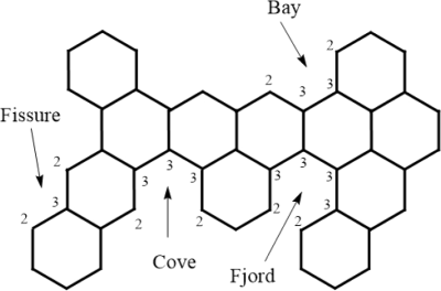

Close

Fig. 1

Instances of a fjord, cove, fissure and a bay in a BS.

Export to PPT

Employing Lemma 3.1 on an arbitrary BS comprising $\upsilon$ vertices, $\tau$ inlets and $\eta$ hexagons, one can calculate $S{C}_{\alpha }$ , $P{C}_{\alpha }$ and $S{O}_{\alpha }$ as follows:

In sections that immediately follow, we evaluate $S{C}_{\alpha }$ , $P{C}_{\alpha }$ and $S{O}_{\alpha }$ for the 30 BHs (chosen test molecules) by utilizing Eqs. (3.8), (3.9), and (3.10) respectively.

4 Optimization problem and algorithm

Following Hayat et al. (2023), we consider the heat capacity $\Delta H$ and the entropy $E$ to be the representatives of thermodynamic properties of a chemical compound. Moreover, we choose the 30 lower benzenoid hydrocarbons (BHs) as our test molecules. Fig. 2 delivers the lower 30 BHs. Table 1 presents the heat capacity $\Delta H$ , the entropy $E$ , the general Randić index $R_{\alpha }$ , the general sum-connectivity index $SC{I}_{\alpha }$ , and the general Sombor index $S{O}_{\alpha }$ of 30 lower BHs.

Let $R\left(\alpha \right)=R_{\alpha }(Y,X)$ be the correlation function between $Y\in \{\Delta H,E\}$ and $X\in \{R_{\alpha },SC{I}_{\alpha },S{O}_{\alpha }\}$ . Then, we formulate the following optimization problem:

Close

Fig. 2

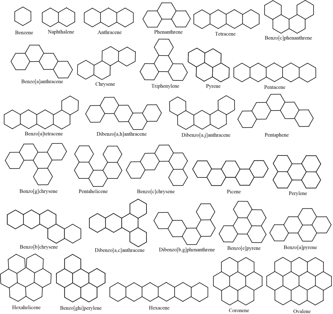
The 30 lower BHs.

Export to PPT

Next, we present the pseudo code of corresponding to the above optimization formulation in Algorithm 1.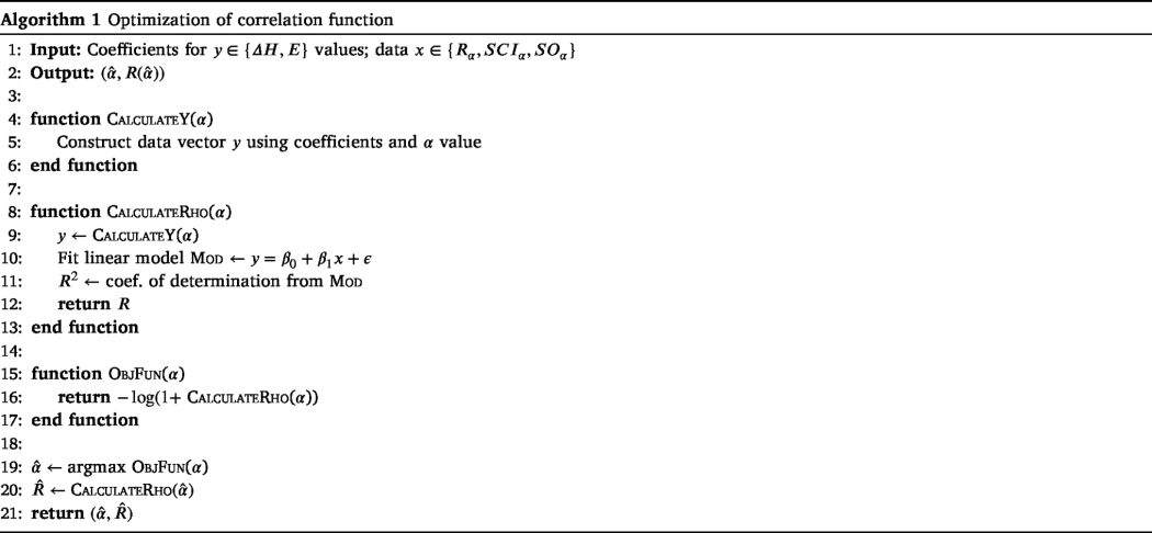

Close

Export to PPT

Note that Algorithm 1 optimizes a correlation function by determining the best value of the parameter $\alpha$ . It constructs a data vector $y$ based on given coefficients and $\alpha$ , then fits a linear model between $y$ and the input data $x$ , calculating the coefficient of determination $R^2$ as a measure of fit. The objective function is defined to minimize $-log(1+R^2)$ , aiming to find the optimal $\alpha$ that maximizes correlation. Finally, the algorithm returns the optimal $\alpha$ and the corresponding $R^2$ value.

5 Computational results

In this section, a robust linear correlation is established between key molecular attributes — such as the number of atoms, molecular weight, and molecular surface area — and the thermodynamic properties, specifically heat capacity ( $\Delta H$ ) and entropy ( $E$ ), for the 30 lower benzenoid hydrocarbons. The study demonstrates that as these the molecular features increase, there is a corresponding rise in both $\Delta H$ and $E$ , underscoring the predictability of thermodynamic properties based on molecular structure. This foundational insight sets the stage for further exploration of how molecular characteristics influence thermodynamic behavior.

Entropy is the thermodynamic function for predicting the spontaneity of a reaction. Whereas, the heat capacity of a substance is defined as the amount of heat required to raise the temperature of a given quantity of the substance by one degree Celsius. Several factors can affect the entropy and heat capacities of the substances, including, number of atoms, molecular weight, volume, molecular surface area, boiling point and melting point (Latimer, 1921; Origlia et al., 2001). As the number of atoms in the system increases, regardless of their masses, its entropy and heat capacity values increase. The higher the boiling point and melting point, the larger entropy and heat capacity of the system. In addition, as the volume or the molecular surface area of the compound increases, the entropy and the heat capacity also increase. The entropies $\left(E\right)$ and heat capacities $\left(\Delta H\right)$ , the molecular formula $\left(MF\right)$ , number of atoms $\left(N_{atoms}\right)$ , molecular weights $\left(MW\right)$ and molecular surface area $\left(MSA\right)$ of the $30$ lower benzenoids are listed in Table 2.

Results obtained show that there are adequate linear correlations between the number of atoms in the molecule $\left(N_{atoms}\right)$ versus the heat capacity (Fig. 3(a)) and the entropy (Fig. 3(b)) with $R^2$ of 0.9994 and 0.9774, respectively. For entropy property, the deviation of the linear correlation is found for $N_{atoms}>36$ . A closer examination of Table 2 reveals that substances with similar molecular formula or number of atoms have almost similar $E$ , and $\Delta H$ values. For examples, systems with $N_{atoms}=30$ , $\Delta H$ value (measured in cal/mol.K) lies in the range from 50.938 to 52.44 with an average of 52.125, while $E$ value (measured in cal/mol.K) is ranged from $105.261-110.0.37$ with an average of 108.055. Additionally, systems with $N_{atoms}=36$ have $\Delta H$ values range from 63.813 to 64.388 with an average of 64.089, while their $E$ values lie in the range from $115.262-123.493$ with an average of 120.773.

A closer examination of Table 2 reveals that smaller molecules with lower molecular weights have lower $E$ and $\Delta H$ values, while the opposite is true. For example, Table 2 shows that the smallest $E$ of 69.028 and $\Delta H$ of 17.151 belong to benzene molecule with molecular weight of 78.048 g/mol. The picture is not similar for larger molecules, Whereas, the maximum $E$ of 84.491 belongs to Ovalene molecule with molecular weight of 398.112 g/mol, while the maximum $\Delta H$ value of 133.95 corresponds to Hexacene with molecular weight of 328.128 g/mol. This deviation in the results of obtained for the larger molecule can be clearly viewed by plotting the linear correlation between the $MW$ versus $E$ and $\Delta H$ values as shown in Fig. 3. The linear correlation coefficient $R^2$ of 0.9862 and 0.9298 are belong, correspondingly, to $\Delta H$ (Fig. 3(a)) and $E$ (Fig. 3(b)) properties. As can be seen in Fig. 3, the deviation of the linear correlation is clearly observed for larger molecules. In addition, the degree of deviation is greater for $E$ property than for the $\Delta H$ one.

Close

Fig. 3

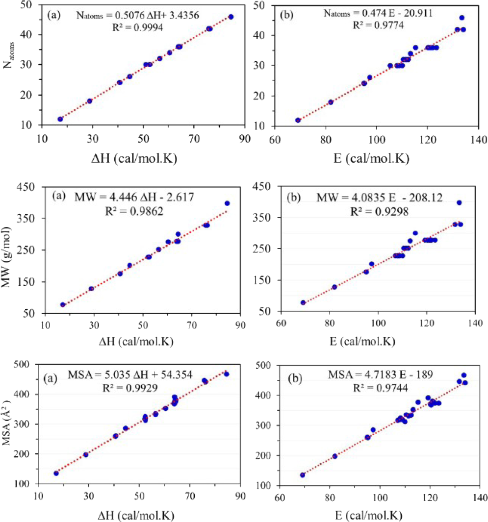
Correlation curves between $N_{atoms}$ , $MW$ and $MSA$ with the chosen properties.

Export to PPT

Fig. 3 shows good linear correlations between the molecular weight $\left(MW\right)$ of the investigated benzenoids and their $\Delta H$ and $E$ values. The linear correlations coefficients $R^2$ of 0.9862 and 0.9298 are belong, correspondingly, to $\Delta H$ (Fig. 3(a)) and $E$ (Fig. 3(b)) properties. As can be seen in Fig. 3, the deviation of the linear correlation is clearly observed for larger molecules. In addition, the degree of deviation is greater for $E$ property than for the $\Delta H$ one.

Fig. 3 shows good linear correlations between the molecular weight $\left(MW\right)$ of the investigated benzenoids and their $\Delta H$ and $E$ values.

The entropy and heat capacity of a substance are also correlated with its molecular surface area (MSA); see Fig. 3 for details. Examination of Table 2 illustrates that the smaller the $MSA$ , the smaller $E$ and $\Delta H$ values. It is found that benzene molecule with the smallest $MSA$ value of 135.58 ${\mathring{A}}^2$ has the smallest $E$ and $\Delta H$ values of 69.028 and 17.151, respectively. On the other hand, Ovalene with the maximum $MSA$ of 467.46 ${\mathring{A}}^2$ has the $E$ and $\Delta H$ values of 133.467 and 84.491, respectively. Notice that, the maximum $E$ value of 133.95 belongs to Hexacene molecule with $MSA$ of 442.77 ${\mathring{A}}^2$ . An excellent linear correlation is found between the $MSA$ and both $E$ and $\Delta H$ properties with $R^2$ of 0.9744 and 0.9929, respectively. Again, the entropies of the larger systems are deviated from these linear relationships.

Optimized geometries of the thirty investigated aromatic hydrocarbon molecules at the $B3LYP/6-31G\left(d\right)$ level of theory in the gas phase computed by Gaussian 09 (Frisch, 2009) and visualized by GaussView 05 (Dennington et al., 2007) software packages as implemented in Aziz supercomputer (http://hpc.kau.edu.sa) at King Abdulaziz University’s High-Performance Computing Centre.

In general, it can be concluded that the entropies and heat capacities of the 30 lower benzenoids are well correlated with the number of atoms, molecular surface area and molecular weights, however, some deviation from the linear correlation is observed for larger systems.

In conclusion, the analyses in the next two subsections offer complementary approaches to predicting thermodynamic properties. This section establishes strong linear correlations based on physical molecular attributes, such as the number of atoms, molecular weight, and surface area. In contrast, the next two subsections refine this understanding by introducing and optimizing mathematical indices ( $R_{\alpha }$ , $SC{I}_{\alpha }$ , and $S{O}_{\alpha }$ ), which more precisely capture these relationships. Together, these studies enhance our understanding of the influence of molecular structure on thermodynamic properties, effectively bridging the gap between direct physical observations and advanced mathematical modeling through graphical indices.

In this section, we present our computational results by employing Algorithm 1 on different computational platforms such as Octave and R Studio. For results from the next subsection, we employed the computational platform Octave.

Note that, in order to be suited for a linear regression analysis the data is supposed to be tested for normality. There are several tests for normality, including Shapiro–Wilk, Lilliefors, and the tests reported in Jäntschi (2019). Other tests such as Anderson–Darling, Cramér-von Mises, Kolmogorov–Smirnov are reported in Jäntschi (2020). Moreover, it is very important to not have outliers and extreme values, since both may leverage your regression.

5.1

5.1 Linear correlation analysis of general graphical indices

The statistical analysis of Figs. 4 and 5 demonstrates the correlation between three general indices ( $R_{\alpha }$ , $SC{I}_{\alpha }$ , and $S{O}_{\alpha }$ ) and the thermodynamic properties of lower benzenoid hydrocarbons, specifically heat capacity $\left(\Delta H\right)$ and entropy $\left(E\right)$ . The curves in these figures show how the correlation coefficients vary with the parameter $\alpha$ . These curves have been generated by using the software Octave. Notably, the optimal $\alpha$ values for $R_{\alpha }$ , $SC{I}_{\alpha }$ , and $S{O}_{\alpha }$ provide strong correlations with both $\Delta H$ and $E$ . For $R_{\alpha }$ , the optimal value is $\alpha =-1.845$ , achieving a correlation coefficient of $\rho =0.997$ with both $\Delta H$ and $E$ . The $SC{I}_{\alpha }$ index is optimal at $\alpha =-0.319$ , with a corresponding correlation coefficient of $\rho =0.997$ . The $S{O}_{\alpha }$ index shows the highest correlation across both properties at $\alpha =-1.067$ , with a correlation coefficient of $\rho =0.998$ , indicating its superior predictive potential. These results emphasize the effectiveness of these indices, particularly $S{O}_{\alpha }$ , when they are properly optimized for the prediction of thermodynamic properties in benzenoid hydrocarbons.

Figs. 4 and 5 provide a magnified view of the regions around the best values of the parameter $\alpha$ for the general indices $R_{\alpha }$ , $SC{I}_{\alpha }$ , and $S{O}_{\alpha }$ when predicting the thermodynamic properties of lower benzenoid hydrocarbons. These figures emphasize the intervals of $\alpha$ where the correlation with the properties is at its peak. Specifically, for predicting heat capacity ( $\Delta H$ ) in Fig. 4, the optimal intervals are approximately $\alpha =[-2,-1.5]$ for $R_{\alpha }$ , $[-0.5,-0.1]$ for $SC{I}_{\alpha }$ , and $[-1.5,-0.5]$ for $S{O}_{\alpha }$ . Similarly, for predicting entropy $\left(E\right)$ in Fig. 5, the best intervals for these indices are also within these ranges: $R_{\alpha }=[-2,-1.5]$ , $SC{I}_{\alpha }=[-0.5,-0.1]$ , and $S{O}_{\alpha }=[-1.5,-0.5]$ .

These intervals represent the ranges of $\alpha$ where each index reaches its highest predictive potential, with the $S{O}_{\alpha }$ index particularly standing out due to its consistent performance across both thermodynamic properties. By focusing on these specific intervals, Figs. 4 and 5 underscore the importance of fine-tuning the parameter $\alpha$ to maximize the predictive accuracy of $R_{\alpha }$ , $SC{I}_{\alpha }$ , and $S{O}_{\alpha }$ indices for estimating the thermodynamic properties of benzenoid hydrocarbons.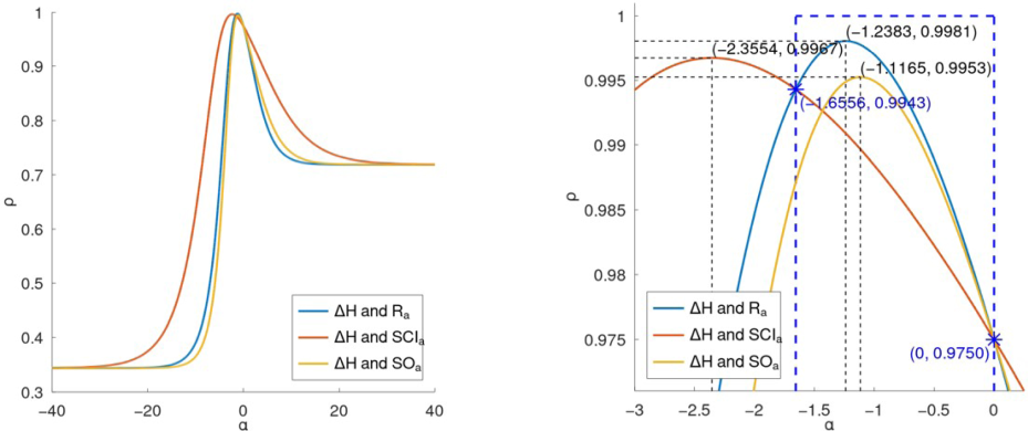

Close

Fig. 4

Far and new views of the correlation curves between general indices and $\Delta H$ of lower benzenoids.

Export to PPT

It has been observed that the optimal $\alpha$ intervals for the three general indices, highlighting the regions above the horizontal dashed lines where the correlation coefficient $\left(\rho \right)$ is strong. For the general Randić index ( $R_{\alpha }$ ), the optimal interval for predicting heat capacity ( $\Delta H$ ) is approximately $[-1.8384,-0.5499]$ , while for entropy $\left[2.5110,1.3334\right]$ . The general sum-connectivity index ( $SC{I}_{\alpha })$ shows strong correlation within the interval $[-3.3914,-1.1480]$ for $\Delta H$ and $[-4.4900,-2.7642]$ for $E$ , indicating its effectiveness within these ranges. The general Sombor index ( $S{O}_{\alpha }$ ) demonstrates the broadest and most stable interval of strong correlation, approximately $[-1.5559,-1.4797]$ for both $\Delta H$ and $E$ , making it the most versatile and reliable predictor across a wider range of $\alpha$ values compared to the other indices. This analysis underscores the importance of selecting the correct $\alpha$ interval for each index to achieve optimal predictive accuracy for thermodynamic properties.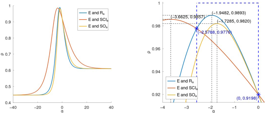

Close

Fig. 5

Far and new views of the correlation curves between general indices and $E$ of lower benzenoids.

Export to PPT

5.2

5.2 Multiple prediction potential of general graphical indices

Note that Section 5 consider the two chosen thermodynamic properties i.e. $\Delta H$ and $E$ individually to investigate their prediction potential with $G{D}_d\in \{S{C}_{\alpha },P{C}_{\alpha },S{O}_{\alpha }\}$ . This section investigate the same problem with $G{D}_d\in \{S{C}_{\alpha },P{C}_{\alpha },S{O}_{\alpha }\}$ and simultaneously choosing both $\Delta H$ and $E$ . In order to perform this study, we employ multivariate regression analysis as we now have more than one independent variables. The multivariate regression analysis has been performed on the statistical environment R Studio.

Let $x_1=\Delta H,x_2=E$ (resp. $y=P{C}_{\alpha }$ ) the two independent variables (resp. dependent variable). Since there are more than one independent variables are involved, we employ multivariate correlation coefficient to investigate the prediction ability of the general product-connectivity index for predicting $\Delta H$ and $E$ . Let $R\left(\alpha \right)=\rho (P{C}_{\alpha };\Delta H,E)$ be the multivariate correlation function between $P{C}_{\alpha }$ and the two chosen properties $\Delta H$ and $E$ . Thus, optimizing $R\left(\alpha \right)$ would deliver us the optimal value(s) of $\alpha$ (let us denote that with $\hat{\alpha }$ ) for which the prediction ability of $P{C}_{\alpha }$ and the two test properties $\Delta H$ and $E$ is the strongest. We apply the following same algorithm as we did in Section 5 by replacing the correlation function with the multivariate correlation function.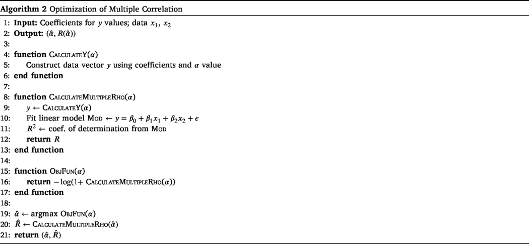

Close

Export to PPT

The main difference between Algorithm 2 and the previous algorithm (Algorithm 1) is the use of multiple independent variables ( $x_1$ and $x_2$ ) in the linear model. In Algorithm 1, the linear model is a simple regression with a single predictor variable $x$ , whereas in Algorithm 2, the linear model is a multiple regression with two predictor variables, $x_1$ and $x_2$ . This modification requires adjusting the calculation of the correlation (specifically $R^2$ ), as Algorithm 2 now considers the combined effect of both predictors on $y$ . The objective function and the optimization process remain similar, aiming to find the optimal $\alpha$ that maximizes the correlation in this multivariate context.

A built-in optimizing tool in $\mathrm{R}$ Studio language is used by applying Algorithm 2 to generate the required $\alpha$ vs $R\left(\alpha \right)$ curves. Fig. 6 depicts such a plot incorporating the bivariate relationship between $R\left(\alpha \right)$ and $\alpha$ delivering $\hat{\alpha }=-0.319$ and the corresponding correlation value of $\rho =0.997$ .

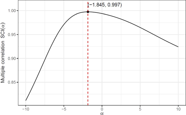
Applying the same computational process and Algorithm 2, we obtain Fig. 7 for the general sum-connectivity index $S{C}_{\alpha }$ . Multiple correlation curve between $R\left(\alpha \right)$ and $\alpha$ show that the optimal value of $\alpha$ is ${\alpha }_{max}=-1.845$ and the corresponding correlation value of $\rho =0.997$ .

Close

Fig. 6

Multiple correlation curve between $R\left(\alpha \right)$ and $\alpha$ delivering $\hat{\alpha }=-0.319$ and the corresponding correlation value of $\rho =0.997$ .

Export to PPT

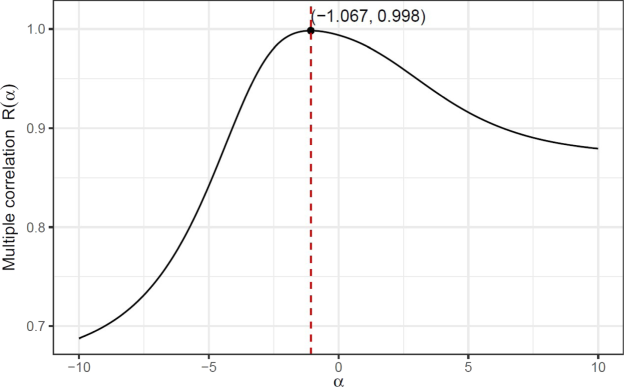
A similar computational process by employing Algorithm 2 deliver Fig. 8 for the general Sombor index $S{O}_{\alpha }$ . Multiple correlation curve between $R\left(\alpha \right)$ and $\alpha$ show that the optimal value of $\alpha$ is ${\alpha }_{max}=-1.067$ and the corresponding correlation value of $\rho =0.998$ .

Close

Fig. 7

Multiple correlation curve between $R\left(\alpha \right)$ and $\alpha$ delivering ${\alpha }_{max}=-1.845$ and the corresponding correlation value of $\rho =0.997$ .

Export to PPT

Close

Fig. 8

Multiple correlation curve between $R\left(\alpha \right)$ and $\alpha$ delivering ${\alpha }_{max}=-1.067$ and the corresponding correlation value of $\rho =0.998$ .

Export to PPT

6 Conclusion

CRediT authorship contribution statement

Suha Wazzan: Writing – review & editing, Validation, Supervision, Resources, Project administration, Methodology. Sakander Hayat: Writing – original draft, Methodology, Formal analysis, Conceptualization. Wafi Ismail: Writing – original draft, Visualization, Validation, Software, Investigation, Formal analysis.

References

- First-principles prediction of enthalpies of formation for polycyclic aromatic hydrocarbons and derivatives. J. Phys. Chem. A.. 2015;119:11329-11365.
- [Google Scholar]
- Topological indices for structure–activity corrections. Top. Curr. Chem.. 1983;114:21-55.
- Quantitative structure–property relationships (QSPRS) for the estimation of vapor pressure: A hierarchical approach using mathematical structural descriptors. J. Chem. Inf. Comput. Sci.. 2001;41(3):692-701.
- New spectral indices for molecular description. MATCH Commun. Math. Comput. Chem.. 2008;60:3-14.
- On benzenoid systems with minimal number of inlets. J. Serb. Chem. Soc.. 2013;78(9):1351-1357.
- GaussView, Version 4.1.2. Shawnee Mission, KS: Semichem Inc.; 2007.
- Molecular Topology. Nova, Huntington; 2001.
- Frisch, A., 2009. Gaussian 09 W Reference. Vol. 25, Wallingford, USA, p. 470.
- Geometric approach to degree-based topological indices: Sombor indices. MATCH Commun. Math. Comput. Chem.. 2021;86(1):11-16.
- Novel Molecular Structure Descriptors – Theory and Applications, Vols. 1 & 2 Kragujevac: Univ. Kragujevac; 2010.
- Mathematical Concepts in Organic Chemistry. New York: Springer-Verlag; 1986.
- Testing the quality of molecular structure descriptors, vertex-degree-based topological indices. J. Serb. Chem. Soc.. 2013;78:805-810.
- Structure-property modeling for thermodynamic properties of benzenoid hydrocarbons by temperature-based topological indices. Ain Shams Eng. J.. 2024;15(3):102586
- Statistical significance of valency-based topological descriptors for correlating thermodynamic properties of benzenoid hydrocarbons with applications. Comput. Theor. Chem.. 2023;1227:114259
- Hyper-zagreb index in fuzzy environment and its application. Heliyon. 2024;10(16):e36110
- Hyper-Wiener index for fuzzy graph and its application in share market. J. Intell. Fuzzy Systems. 2021;41(1):2073-2083.
- Multiplicative version of first zagreb index in fuzzy graph and its application in crime analysis. Proc. Natl. Acad. Sci. India A. 2024;94(1):127-141.
- Neighbourhood and competition graphs under fuzzy incidence graph and its application. Comput. Appl. Math.. 2024;43(7):411.
- A test detecting the outliers for continuous distributions based on the cumulative distribution function of the data being tested. Symmetry. 2019;11(6):835.
- Detecting extreme values with order statistics in samples from continuous distributions. Mathematics. 2020;8(2):216.
- Interpretation of quantitative structure- property and- activity relationships. J. Chem. Inf. Comput. Sci.. 2001;41(3):679-685.
- Topological indices and graph entropies for carbon nanotube Y-junctions. J. Math. Chem.. 2024;62(1):73-108.
- Topological indices of lead sulphide using polynomial technique. Mol. Phys.. 2024;122(3):e2249131
- The mass effect in th entropy of solids and gases. J. Am. Chem. Soc.. 1921;43(4):818-826.
- Face index of silicon carbide structures: An alternative approach. Silicon. 2024;16:5865-5876.
- Apparent molar volumes and apparent molar heat capacities of aqueous solutions ofn, N-dimethylformamide and n, N-dimethylacetamide at temperatures from 278.15 to 393.15 K and at the pressure 0.35 MPa. J. Chem. Thermodyn.. 2001;33(8):917-927.
- Vertex-edge partition resolvability for certain carbon nanocones. Polycycl. Aromat. Compd.. 2024;44(3):1745-1759.
- Molecular Descriptors for Chemoinformatics, Vols. 1 & 2. Weinheim, Germany: Wiley-VCH; 2009.
- Symmetry-adapted domination indices: The enhanced domination sigma index and its applications in QSPR studies of octane and its isomers. Symmetry. 2023;15(6):1202.
- Advancing computational insights: Domination topological indices of polysaccharides using special polynomials and QSPR analysis. Contemp. Math.. 2024;5(1):26-49.
- Unveiling novel eccentric neighborhood forgotten indices for graphs and gaph operations: A comprehensive exploration of boiling point prediction. AIMS Math.. 2024;9(1):1128-1165.
- Structural determination of the paraffin boiling points. J. Am. Chem. Soc.. 1947;69:17-20.
- A survey on graphs extremal with respect to distance-based topological indices. MATCH Commun. Math. Comput. Chem.. 2014;71:461-508.