On the thermal analysis of magnetohydrodynamic Jeffery fluid via modern non integer order derivative

Kashif Ali Abro; Irfan Ali Abro; Sikandar Mustafa Almani; Ilyas Khan

doi:10.1016/j.jksus.2018.07.012

View/Download PDF

Buy Reprints

PDF

Translate this page into:

Original article

31 (

); 973-979

doi:

10.1016/j.jksus.2018.07.012

On the thermal analysis of magnetohydrodynamic Jeffery fluid via modern non integer order derivative

Kashif Ali Abro^{^a,⁎}, Irfan Ali Abro^{^b}, Sikandar Mustafa Almani^{^c}, Ilyas Khan^{^d}

a Department of Basic Sciences and Related Studies, Mehran University of Engineering Technology, Jamshoro, Pakistan

b Department of Metallurgy and Materials, Mehran University of Engineering Technology, Jamshoro, Pakistan

c Université de Nantes-GEPEA Lab, CNRS-UMR 6144, Saint Nazaire Cedex, France

d Basic Engineering Sciences Department College of Engineering, Majmaah University, P.O.Box 66, Majmaah 11952 Saudi Arabia

⁎Corresponding author. kashif.abro@faculty.muet.edu.pk (Kashif Ali Abro)

Received: 2018-6-13, Accepted: 2018-7-9, Published: 2018-10-01

Disclaimer:
This article was originally published by Elsevier and was migrated to Scientific Scholar after the change of Publisher.

Peer review under responsibility of King Saud University.

Abstract

The uniqueness of thermal radiation effects on materials has an adhesive role in engineering. This article emphasizes the effects of thermal radiation of Jeffery fluid with magnetic field by employing Caputo-Fabrizio fractional derivative. Analytical solutions for the velocity field and temperature distribution are based on integral transforms (Fourier Sine and Laplace transform) with their inversion. The general solutions have been established in terms of elementary functions and product of convolution theorem satisfying initial and boundary conditions. This analysis is one of the infrequent contributions to elucidate the rheology of Jeffery fluid for free convective problem on oscillating plate. In order to bring physical insights, four models have been prepared for comparison i-e (i) Jeffery fluid with magnetic field (ii) Jeffery fluid without magnetic field (iii) Second grade fluid with magnetic field and (iv) Second grade fluid without magnetic field for several rheological parameters for instance, viscosity $ν$ , thermal radiation $Rd$ , thermal conductivity $k$ , Jeffrey fluid parameter $λ$ , Hartmann number $H_{a}$ , magnetic field $M$ , Prandtl number $P_{r}$ , Grashof number on fluid flow. At the end, our results suggested that Ordinary Jeffery fluid with magnetic field oscillates more rapidly to remaining models of fluid but fractionalized Jeffery fluid with magnetic field has reciprocal behavior of fluid flow.

Keywords

Thermal radiation

Jeffery fluid

Caputo-Fabrizio fractional derivative

Fourier Sine and Laplace transform

Show Related Articles from PubMed

1 Introduction

The computational and physico-mathematical analysis in non-Newtonian fluid has diverted the attention of various researchers; this is due to broad applications of certain fluids in engineering such as industrial adhesives and lubricants (Ver Strate and Struglinski, 1991), gels, drugs and creams (Suryawanshi et al., 2012), plastics fabrication (Balmforth and Craster, 1999), and also ecological systems comprising hyper-concentrated sediments, mud flows, contaminant release and oil spills (Jokuty et al., 1995). The conventional Navier-Stokes viscous model (Newtonian) invalidates non-Newtonian fluids due to intrinsic properties. Newtonian fluid is insufficient to describe the dynamics and rheological phenomenon of many fluids for instance, Weissenberg effects, shear-thinning/thickening, stress differences, fading memory, spurt, yield stress, elongation, retardation, relaxation, re-coil, micro-structure and several others. Different models have been proposed to characterize the rheology of non-Newtonian fluid few of them are; Burgers elasto-viscous fluid model (Tripathi and Anwar Bég, 2014), Sisko’s model (Sisko, 1958), differential third and second grade fluid models (Reiner-Rivlin) (Sahoo and Poncet, 2011; Sarpkaya and Rainey, 1971), Oldroyd-B fluid model (Khan et al., 2012), Maxwell fluid model (Abro et al., 2015; Abro and Shaikh, 2015), Jeffery’s model (Qasim, 2013). The Jeffery fluid model is viscoelastic non-Newtonian fluid that exhibits retardation and relaxation phenomenon. The Jeffery fluid model is simpler linear model in which convective derivative is omitted for time derivative. For this cause, several investigations have been carried on Jeffery fluid few of them are hereby cited. Hayat and et al. have traced out Jeffrey fluid for unsteady mixed convection flow under the existence of thermal radiation over a stretching sheet (Hayat and Mustafa, 2010). The Jeffrey fluid for stagnation point flow on unsteady oscillations has been analyzed by Nadeem et al. (2014). Hayat et al. (2012) have investigated the flow of Jeffery fluid in the presence and absence of radiation under the influences of heat source and power law heat flux. Shehzad et al. (2013) worked out on the radiative flow of Jeffrey fluid under impacts of joule heating and thermophoresis with mixed convection. Khan (2015) examined effects the unsteady free convection flow of a Jeffrey fluid and traced out an exact solution. Dalir (2014) investigated heat transfer and convection flow of a Jeffrey fluid with entropy generation over a stretching sheet using Numerical study. Hayat et al. (2010) worked on fractionalized Oscillatory and rotational flows of Jeffrey fluid in porous medium. Idowu et al. (2013) emphasized the impacts of unsteady magnetohydrodynamic flow of Jeffrey fluid with chemical reaction, mass and heat transfer in a horizontal channel. Off course, the study can be continued but we end here by citing few recent studies on magnetic field (Abro and Solangi, 2017; Sheikholeslami and Rokni, 2018; Abro et al., 2018; Atangana and Koca, 2016; Abro et al., 2017 ), thermal radiation (Abro et al., 2018; Khan and Abro, 2018), Porous medium (Abro et al., 2017; Abro et al., 2017), heat and mass transfer (Atangana, 2016; Sheikholeslami et al., 2018; Abro and Khan, 2017; Sheikholeslami et al., 2018; Abro et al., 2018; Mohyud-Din et al., 2015; Khan et al., 2017 ), nanofluids (Sheikholeslami et al., 2018; Sheikholeslami et al., 2018; Khan et al., 2017 ) and modern fractional derivatives (Al-Mdallal et al., 2018; Saad et al., 2017; Abro et al., 2018; Atangana and Baleanu, 2017; Laghari et al., 2017 ). Motivating by all mentioned models, our aim is to emphasize the effects of oscillating flow of Jeffery fluid for magnetic field and thermal radiation by employing Caputo-Fabrizio fractional derivative. Analytical solutions for the velocity field and temperature distribution are based on integral transforms (Fourier Sine and Laplace transform). The general solutions have been established in terms of elementary functions and product of convolution theorem satisfying initial and boundary conditions. This analysis is one of the infrequent contributions to elucidate the rheology of Jeffery fluid for free convective problem on oscillating plate. In order to bring physical insights, four models have been prepared for comparison i-e (i) Jeffery fluid with magnetic field (ii) Jeffery fluid without magnetic field (iii) Second grade fluid with magnetic field and (iv) Second grade fluid without magnetic field for several rheological parameters for instance, viscosity $ν$ , thermal radiation $Rd$ , thermal conductivity $k$ , Jeffrey fluid parameter $λ$ , Hartmann number $H_{a}$ , magnetic field $M$ , Prandtl number, $P_{r}$ , Grashof number on fluid flow (see Fig. 1).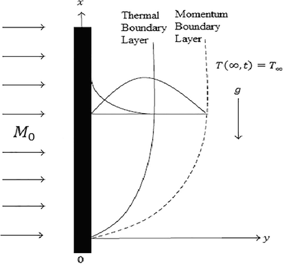

Geometry of Jeffery Fluid for Vertical Plate.

2 Governing equations

The governing equation which describes unsteady incompressible flow

(1)

\nabla . V = 0, div T + ρ g + J \times M = ((V . \nabla) V + \frac{\partial V}{\partial t}) ρ,

(2)

Curl M = J μ_{m}, Curl E = - \frac{\partial M}{\partial t}, \nabla . M = 0,

In Eqs. (1) and (2),

V

T

ρ

g

J

J μ_{m}

E

velocity field, Cauchy stress tensor, density of fluid, gravitational force, current density, total magnetic field, magnetic permeability and total electric field current. The constitutive equations for Jeffrey fluid are described below

(3)

T = - pI + S, \frac{(1 + λ_{1}) S}{μ} = (\frac{\partial A_{1}}{\partial t} + (V . \nabla) A_{1}) λ_{2} + A_{1},

where,

- pI

S

λ_{1}

μ

A_{1}

and

λ_{2}

indeterminate part of the stress, extra tensor, ratio of relaxation to retardation times, dynamic viscosity, Rivlin-Ericksen tensor and retardation time of Jeffery fluid. We assume the stress and velocity field for the oscillating flow as below

(4)

V = V (y, t) = V (y, t) i, S = S (y, t),

where,

i

unit vector along the ??-direction and

w

is ??-component of velocity

V

of the Cartesian coordinate system. The stress field fulfills the assumption

S (y, 0 = 0)

which generates the below equation

(5)

S_{xz} = S_{zx} = S_{yz} = S_{zy} = S_{zz} = S_{xx} = 0, (1 + λ_{2} \frac{\partial}{\partial t}) \frac{\partial V}{\partial t} = S_{xy} \frac{(1 + λ_{1})}{μ},

where,

S_{xy}

is the non-trivial tangential stress. Assume the impact of thermal radiation along with electrically conducting flow of Jeffery fluid about the vertical plate located in

xz

-plane. It is assumed at time

t = 0^{+}

, the temperature of plate raised up and the constant temperature

T_{w}

is kept up at

t > t_{0}

. At time

t ⩽ 0

, the fluid and plate are at rest in the constant temperature

T_{\infty}

and when

t ⩽ t_{0}

, lowered at

T_{\infty} + (T_{w} - T_{\infty}) (t / t_{0})

. Using usual Boussinesq approximations and implementing above assumptions, the energy and momentum equations for electrically conducting flow of Jeffery fluid in porous medium about the vertical plate as (Khan, 2015; Zin et al., 2016)

(6)

(1 + λ_{2} \frac{\partial}{\partial t}) \frac{\partial^{2} V}{\partial y^{2}} = (1 + λ_{1}) \frac{ρ}{μ} \frac{\partial V}{\partial t} - σ M_{0}^{2} V + ρ g β (T - T_{\infty}),

(7)

\frac{k}{ρ c_{p}} \frac{\partial^{2} V}{\partial y^{2}} = \frac{\partial T}{\partial t} - \frac{\partial q_{r}}{\partial y},

while, initial and boundary conditions are

(8)

T (y, 0) = T_{\infty}, V (y, 0) = 0, y > 0,

(9)

T (0, t) = T_{w}, t ⩾ t_{0}, V (0, t) = UH (t) \cos (ω t) or U \sin (ω t), t > 0,

(10)

T (\infty, t) = T_{\infty}, V (\infty, t) = 0, t > 0,

where,

V

T

ρ

g

c_{p}

k

T_{w}

T_{\infty}

q_{r}

are fluid velocity, temperature, constant density, acceleration due to gravity, specific heat capacity, thermal conductivity, wall temperature, free stream temperature and radiation heat flux, respectively. While radiation heat flux can be written by using Rosseland approximation as

(11)

4 σ^{*} \frac{\partial^{4} T}{\partial y} = - 3 k_{1} q_{r},

where,

σ^{*}, k_{1}

are Stefan-Boltzmann and absorption coefficient respectively. Temperature differences for flow are assumed sufficiently small and simplifying Eq. (7), we obtained that

(12)

\frac{\partial^{2} T (y, t)}{\partial y^{2}} (1 + \frac{16 T_{\infty}^{3} σ^{*}}{3 k_{1} k}) = \frac{\partial T}{\partial y} \frac{ρ c_{p}}{k},

Implementing dimensionless numbers and variables,

(13)

t^{*} = \frac{U_{0}^{2} t}{ν}, V^{*} = \frac{V}{U_{0}}, y^{*} = \frac{U_{0} y}{ν}, Rd = \frac{16 T_{\infty}^{3} σ^{*}}{3 k_{1} k}, λ = \frac{U_{0}^{2} λ_{2}}{ν}, T = \frac{T - T_{\infty}}{T_{w} - T_{\infty}}, H_{a} = \frac{ν M_{0}^{2} σ}{U_{0}^{2} ρ}, P_{r} = \frac{c_{p} μ}{k}, G_{r} = \frac{ν β g (T_{w} - T_{\infty})}{U_{0}^{3}} .

where, $t$ , $w$ , $U$ , $ν$ , $y$ , $Rd$ , $T$ , $σ$ , $k_{1}$ , $k$ , $λ$ , $H_{a}$ , $M$ , $P_{r}$ , $G_{r}$ are the time, velocity distribution, Non-zero parameter, viscosity, spatial variable, thermal radiation, temperature, Stefan-Boltzmann, absorption coefficient, thermal conductivity, Jeffrey fluid parameter, Hartmann number, magnetic field, Prandtl number, Grashof number respectively. The corresponding governing differential equations and initial and boundary conditions from Eqs. (6)-(10) are termed as

(14)

(1 + λ_{1}) (D_{t}^{ζ} V (y, t) + H_{a} V (y, t) - G_{r} T (y, t)) = (λ D_{t}^{ζ} + 1) \frac{\partial^{2} V (y, t)}{\partial y^{2}},

(15)

\frac{p_{r}}{(Rd + 1)} D_{t}^{ζ} T (y, t) = \frac{\partial^{2} T (y, t)}{\partial y^{2}},

(16)

T (y, 0) = 0, V (y, 0) = 0, y > 0,

(17)

T (0, t) = t, t > 0, V (0, t) = U H (t) \cos (ω t) or U \sin (ω t), t > 0,

(18)

T (\infty, t) = 0, V (\infty, t) = 0, t > 0 .

where,

D_{t}^{ζ}

is time-fractional derivatives, represents Caputo-Fabrizio fractional derivative operator (time derivative of non-integer order derivative without singular kernel) of order

0 ⩽ ζ ⩽ 1

as in literature earlier published paper (Caputo and Fabrizio, 2015; Shah and Khan, 2016; Zafar and Fetecau, 2016 ) defined as

(19)

D_{t}^{ζ} = \int_{0}^{t} \frac{G^{'} (η)}{1 - ζ} Exp (- \frac{ζ (t - η)}{1 - ζ}) d η, for 0 ⩽ ζ ⩽ 1 .

3 Profile of temperature distribution via Fourier Sine transform

Employing Fourier Sine Transform on fractionalized differential equation, Multiplying both sides of (15) $\sqrt{\frac{2}{π}} \sin (y ψ)$ , integrating the result with respect to y from 0 to infinity (Abro et al., 2016), and considering Eq. (16)₁ in mind the initial and boundary condition, we obtain

(20)

\frac{p_{r}}{(Rd + 1)} D_{t}^{ζ} T_{s} (ψ, t) = (- ψ^{2} T_{s} (ψ, t) + ψ \sqrt{\frac{2}{π}} T (0, t)),

where, The image of Fourier Sine transform of

T (y, t)

T_{s} (ψ, t)

has satisfy Fourier Sine transform defined as

(21)

T_{s} (ψ, t) = \sqrt{\frac{2}{π}} \int_{0}^{\infty} T (y, t) \sin (y ψ) dy,

Implementing Laplace transform on Eq. (20) and (1618)₁, we get

(22)

{\bar{T}}_{s} (ψ, t) = \sqrt{\frac{2}{π}} \frac{(Rd + 1) (δ ζ + s)}{s^{2} {s (P_{r} δ + ψ + ψ Rd) + (ψ δ ζ + ψ Rd δ ζ)}},

where, utilizing the fact

δ = \frac{1}{(1 - ζ)}

we recovered

L {D_{t}^{ζ} T_{s} (ψ, t)} = \frac{δ s}{s + δ ζ}

{\bar{T}}_{s} (ψ, s)

. Now we rewrite Eq. (22) for more suitable presentation, we have

(23)

{\bar{T}}_{s} (ψ, s) = \frac{1}{ψ} \sqrt{\frac{2}{π}} [\frac{1}{s^{2}} - \frac{P_{r} δ}{s {s (P_{r} δ + ψ + ψ Rd) + (ψ δ ζ + ψ Rd δ ζ)}}],

Inverting Eq. (23) by Fourier Sine transform, we obtain

(24)

\bar{T} (y, s) = \frac{2}{π} \int_{0}^{\infty} \frac{\sin (y ψ)}{ψ} [\frac{1}{s^{2}} - \frac{P_{r} δ}{s {s (P_{r} δ + ψ + ψ Rd) + (ψ δ ζ + ψ Rd δ ζ)}}] d ψ,

Finally, in order to trace out the final solution of temperature distribution, we apply inverse Laplace transform on Eq. (24) and employing the fact of integral

\int_{0}^{\infty} \frac{\sin (y λ_{1})}{λ_{1}} d λ_{1} = \frac{π}{2}, y > 0

(Abro, 2016), we attain

(25)

T (y, t) = t - \frac{2 P_{r} δ}{π} \int_{0}^{\infty} \frac{\sin (y ψ)}{ψ (ψ δ ζ + ψ Rd δ ζ)} [1 - Exp (- \frac{P_{r} δ + ψ + ψ Rd}{ψ δ ζ + ψ Rd δ ζ}) t] d ψ .

4 Profile of velocity field via Fourier Sine transform

The case of cosine oscillation $V (0, t) = UH (t) \cos (ω t)$ Employing Fourier Sine Transform on fractionalized differential equation, Multiplying both sides of (14) $\sqrt{\frac{2}{π}} \sin (y ψ)$ , integrating the result with respect to y from 0 to infinity, and considering equation (16)₂ in mind the initial and boundary condition, we obtain

(26)

(1 + λ_{1}) (D_{t}^{ζ} V_{s} (ψ, t) + H_{a} V_{s} (ψ, t) - G_{r} T_{s} (ψ, t)) = (λ D_{t}^{ζ} + 1) (- ψ^{2} V_{s} (ψ, t) + ψ \sqrt{\frac{2}{π}} V (0, t)),

Implementing Laplace transform on equations (26) and (1618)₂, we get

(27)

{\bar{V}}_{s} (ψ, s) = \sqrt{\frac{2}{π}} \frac{U ψ s (δ ζ + s)}{(s^{2} + ω^{2}) ({ss}_{1} + (δ ζ + s) s_{2})} + \sqrt{\frac{2}{π}} \frac{U λ ψ δ s^{2}}{(s^{2} + ω^{2}) ({ss}_{1} + (δ ζ + s) s_{2})} + \sqrt{\frac{2}{π}} \frac{G_{r} (Rd + 1) {(δ ζ + s)}^{2} (1 + λ_{1})}{s^{2} ({ss}_{3} + s_{4}) ({ss}_{1} + (δ ζ + s) s_{2})},

where,

s_{1} = δ + δ λ_{1} + λ δ ψ^{2}

s_{2} = ψ^{2} + (H_{a} + Φ) (1 + λ_{1})

s_{3} = P_{r} δ + ψ + ψ Rd

and

s_{4} = ζ δ ψ + ψ Rd ζ δ

altering Eq. (27) for more suitable presentation and inverting Eq. (27) by means of Fourier Sine transform, we get

(28)

\bar{V} (y, s) = \frac{Us}{s^{2} + ω^{2}} + \frac{2}{π} \int_{0}^{\infty} \frac{\sin (y ψ)}{ψ} \frac{U ψ s (δ ζ + s)}{(s^{2} + ω^{2}) ({ss}_{1} + (δ ζ + s) s_{2})} d ψ + \frac{2}{π} \int_{0}^{\infty} \sin (y ψ) \frac{U λ ψ δ s^{2}}{(s^{2} + ω^{2}) ({ss}_{1} + (δ ζ + s) s_{2})} d ψ + \frac{2}{π} \int_{0}^{\infty} \sin (y ψ) \frac{G_{r} (Rd + 1) {(δ ζ + s)}^{2} (1 + λ_{1})}{s^{2} ({ss}_{3} + s_{4}) ({ss}_{1} + (δ ζ + s) s_{2})} d ψ,

simplifying Eq. (28) by letting

s_{5} = \frac{ζ δ ψ^{2} - ζ δ s_{2}}{ψ^{2} - s_{1} - s_{2}}

s_{6} = \frac{ζ δ s_{2}}{s_{1} + s_{2}}

and

s_{7} = \frac{s_{4}}{s_{3}}

, we investigated following expression for convolution product as

(29)

\bar{V} (y, s) = \frac{Us}{s^{2} + ω^{2}} + \frac{2 (ψ^{2} - s_{1} - s_{2})}{π (s_{1} + s_{2})} \int_{0}^{\infty} \frac{\sin (y ψ)}{ψ} \frac{s (s + s_{5})}{(s^{2} + ω^{2}) (s + s_{6})} d ψ + \frac{2 U λ δ}{π (s_{1} + s_{2})} \int_{0}^{\infty} ψ \sin (y ψ) \frac{s^{2}}{(s^{2} + ω^{2}) (s + s_{6})} d ψ + \frac{2 G_{r} (1 + λ_{1}) (Rd + 1)}{π (s_{1} + s_{2}) s_{3}} \int_{0}^{\infty} \sin (y ψ) \frac{1}{s^{2}} {\frac{{(δ ζ + s_{6})}^{2}}{(s_{7} - s_{6}) (s - s_{6})} + \frac{{(δ ζ + s_{7})}^{2}}{(s_{6} - s_{7}) (s - s_{7})}} d ψ,

Applying inverse Laplace transform on Eq. (30), we have final form of velocity field in term of integral form as

(30)

V (y, t) = UH (t) \cos ω t + \frac{2 UH (t) (ψ^{2} - s_{1} - s_{2})}{π (s_{1} + s_{2})} \int_{0}^{\infty} \int_{0}^{t} \frac{\sin (y ψ)}{ψ} \cos ω (t - q) (s_{5} - s_{6}) Exp (- s_{6}) t d ψ dq + \frac{2 U λ δ s_{7}}{π (s_{1} + s_{2})} \int_{0}^{\infty} \int_{0}^{t} ψ \sin (y ψ) \cos ω (t - q) Exp (- s_{6}) t d ψ dq + \frac{2 G_{r} (1 + λ_{1}) (Rd + 1)}{π (s_{1} + s_{2}) s_{3}} \int_{0}^{\infty} \int_{0}^{t} \sin (y ψ) \times (t - q) \{\frac{{(δ ζ + s_{6})}^{2}}{(s_{7} - s_{6})} Exp (- s_{6}) t + \frac{{(δ ζ + s_{7})}^{2}}{(s_{6} - s_{7})} Exp (- s_{7}) t\} d ψ dq .

Having an identical procedure, we also investigated the case of sine oscillation

V (0, t) = UH (t) \sin (ω t)

by letting the

s_{8} = \frac{ζ δ ψ^{2} - ζ δ s_{2}}{ψ^{2} - 2 s_{1}}

, we recovered the following expression

(31)

V (y, t) = UH (t) \sin ω t + \frac{2 UH (t) (ψ^{2} - 2 s_{1})}{π (s_{1} + s_{2})} \int_{0}^{\infty} \int_{0}^{t} \frac{\sin (y ψ)}{ψ} \sin ω (t - q) (s_{8} - s_{6}) Exp (- s_{6}) t d ψ dq + \frac{2 U λ δ s_{7} ω}{π (s_{1} + s_{2})} \int_{0}^{\infty} \int_{0}^{t} ψ \sin (y ψ) \cos ω (t - q) Exp (- s_{6}) t d ψ dq + \frac{2 G_{r} (1 + λ_{1}) (Rd + 1)}{π (s_{1} + s_{2}) s_{3}} \int_{0}^{\infty} \int_{0}^{t} \sin (y ψ) \times (t - q) {\frac{{(δ ζ + s_{6})}^{2}}{(s_{7} - s_{6})} Exp (- s_{6}) t + \frac{{(δ ζ + s_{7})}^{2}}{(s_{6} - s_{7})} Exp (- s_{7}) t} d ψ dq .

5 Limiting cases

5.1

5.1 Temperature distribution and velocity field without the effects of radiation when $Rd = 0$

The solutions of temperature distribution and velocity field without the effects of radiation cab be recovered by letting $Rd = 0$ in equations (25) and (30), (31) obtained by (Khan, 2015)

(32)

T (y, t) = t - \frac{2 P_{r}}{π} \int_{0}^{\infty} \frac{\sin (y ψ)}{ψ^{2} ζ} [1 - Exp (- \frac{P_{r} δ + ψ}{ψ δ ζ}) t] d ψ .

(33)

V (y, t) = UH (t) \cos ω t + \frac{2 UH (t) (ψ^{2} - s_{1} - s_{2})}{π (s_{1} + s_{2})} \int_{0}^{\infty} \int_{0}^{t} \frac{\sin (y ψ)}{ψ} \cos ω (t - q) (s_{5} - s_{6}) Exp (- s_{6}) t d ψ dq + \frac{2 U λ δ s_{7}}{π (s_{1} + s_{2})} \int_{0}^{\infty} \int_{0}^{t} ψ \sin (y ψ) \cos ω (t - q) Exp (- s_{6}) t d ψ dq + \frac{2 G_{r} (1 + λ_{1})}{π (s_{1} + s_{2}) s_{3}} \int_{0}^{\infty} \int_{0}^{t} \sin (y ψ) \times (t - q) {\frac{{(δ ζ + s_{6})}^{2}}{(s_{7} - s_{6})} Exp (- s_{6}) t + \frac{{(δ ζ + s_{7})}^{2}}{(s_{6} - s_{7})} Exp (- s_{7}) t} d ψ dq .

(34)

V (y, t) = UH (t) \sin ω t + \frac{2 UH (t) (ψ^{2} - 2 s_{1})}{π (s_{1} + s_{2})} \int_{0}^{\infty} \int_{0}^{t} \frac{\sin (y ψ)}{ψ} \sin ω (t - q) (s_{8} - s_{6}) Exp (- s_{6}) t d ψ dq + \frac{2 U λ δ s_{7} ω}{π (s_{1} + s_{2})} \int_{0}^{\infty} \int_{0}^{t} ψ \sin (y ψ) \cos ω (t - q) Exp (- s_{6}) t d ψ dq + \frac{2 G_{r} (1 + λ_{1})}{π (s_{1} + s_{2}) s_{3}} \int_{0}^{\infty} \int_{0}^{t} \sin (y ψ) \times (t - q) {\frac{{(δ ζ + s_{6})}^{2}}{(s_{7} - s_{6})} Exp (- s_{6}) t + \frac{{(δ ζ + s_{7})}^{2}}{(s_{6} - s_{7})} Exp (- s_{7}) t} d ψ dq .

where,

s_{1} = δ + δ λ_{1} + λ δ ψ^{2}

s_{2} = ψ^{2} + (H_{a} + Φ) (1 + λ_{1})

s_{3} = P_{r} δ + ψ

s_{4} = ζ δ ψ

s_{5} = \frac{ζ δ ψ^{2} - ζ δ s_{2}}{ψ^{2} - s_{1} - s_{2}}

s_{6} = \frac{ζ δ s_{2}}{s_{1} + s_{2}}

and

s_{7} = \frac{s_{4}}{s_{3}}

and

s_{8} = \frac{ζ δ ψ^{2} - ζ δ s_{2}}{ψ^{2} - 2 s_{1}} .

5.2

5.2 Velocity field without the effects of magnetic field when $H_{a} = 0 .$

The solutions of velocity field without the effects of transverse magnetic field cab be investigated by employing $H_{a} = 0$ in Eqs. (30) and (31)

(35)

V (y, t) = UH (t) \cos ω t + \frac{2 UH (t) (ψ^{2} - s_{1} - s_{2})}{π (s_{1} + s_{2})} \int_{0}^{\infty} \int_{0}^{t} \frac{\sin (y ψ)}{ψ} \cos ω (t - q) (s_{5} - s_{6}) Exp (- s_{6}) t d ψ dq + \frac{2 U λ δ s_{7}}{π (s_{1} + s_{2})} \int_{0}^{\infty} \int_{0}^{t} ψ \sin (y ψ) \cos ω (t - q) Exp (- s_{6}) t d ψ dq + \frac{2 G_{r} (1 + λ_{1}) (Rd + 1)}{π (s_{1} + s_{2}) s_{3}} \int_{0}^{\infty} \int_{0}^{t} \sin (y ψ) \times (t - q) {\frac{{(δ ζ + s_{6})}^{2}}{(s_{7} - s_{6})} Exp (- s_{6}) t + \frac{{(δ ζ + s_{7})}^{2}}{(s_{6} - s_{7})} Exp (- s_{7}) t} d ψ dq .

(36)

V (y, t) = UH (t) \sin ω t + \frac{2 UH (t) (ψ^{2} - 2 s_{1})}{π (s_{1} + s_{2})} \int_{0}^{\infty} \int_{0}^{t} \frac{\sin (y ψ)}{ψ} \sin ω (t - q) (s_{8} - s_{6}) Exp (- s_{6}) t d ψ dq + \frac{2 U λ δ s_{7} ω}{π (s_{1} + s_{2})} \int_{0}^{\infty} \int_{0}^{t} ψ \sin (y ψ) \cos ω (t - q) Exp (- s_{6}) t d ψ dq + \frac{2 G_{r} (1 + λ_{1}) (Rd + 1)}{π (s_{1} + s_{2}) s_{3}} \int_{0}^{\infty} \int_{0}^{t} \sin (y ψ) \times (t - q) \{\frac{{(δ ζ + s_{6})}^{2}}{(s_{7} - s_{6})} Exp (- s_{6}) t + \frac{{(δ ζ + s_{7})}^{2}}{(s_{6} - s_{7})} Exp (- s_{7}) t\} d ψ dq .

where,

s_{1} = δ + δ λ_{1} + λ δ ψ^{2}

s_{2} = ψ^{2}

s_{3} = P_{r} δ + ψ + ψ Rd

and

s_{4} = ζ δ ψ + ψ Rd ζ δ

s_{5} = \frac{ζ δ ψ^{2} - ζ δ s_{2}}{ψ^{2} - s_{1} - s_{2}}

s_{6} = \frac{ζ δ s_{2}}{s_{1} + s_{2}}

s_{7} = \frac{s_{4}}{s_{3}}

and

s_{8} = \frac{ζ δ ψ^{2} - ζ δ s_{2}}{ψ^{2} - 2 s_{1}} .

5.3

5.3 Velocity field for Second grade fluid with magnetic field when $λ_{1} = 0$ and $H_{a} \neq 0 .$

The solutions of velocity field with the effects of transverse magnetic field for second grade fluid can be traced out by employing $λ_{1} = 0$ and $H_{a} \neq 0$ in Eqs. (30) and (31) obtained by (Samiulhaq et al., 2014)

(37)

V (y, t) = UH (t) \cos ω t + \frac{2 UH (t) (ψ^{2} - s_{1} - s_{2})}{π (s_{1} + s_{2})} \int_{0}^{\infty} \int_{0}^{t} \frac{\sin (y ψ)}{ψ} \cos ω (t - q) (s_{5} - s_{6}) Exp (- s_{6}) t d ψ dq + \frac{2 U λ δ s_{7}}{π (s_{1} + s_{2})} \int_{0}^{\infty} \int_{0}^{t} ψ \sin (y ψ) \cos ω (t - q) Exp (- s_{6}) t d ψ dq + \frac{2 G_{r} (1 + λ_{1}) (Rd + 1)}{π (s_{1} + s_{2}) s_{3}} \int_{0}^{\infty} \int_{0}^{t} \sin (y ψ) \times (t - q) \{\frac{{(δ ζ + s_{6})}^{2}}{(s_{7} - s_{6})} Exp (- s_{6}) t + \frac{{(δ ζ + s_{7})}^{2}}{(s_{6} - s_{7})} Exp (- s_{7}) t\} d ψ dq .

(38)

V (y, t) = UH (t) \sin ω t + \frac{2 UH (t) (ψ^{2} - 2 s_{1})}{π (s_{1} + s_{2})} \int_{0}^{\infty} \int_{0}^{t} \frac{\sin (y ψ)}{ψ} \sin ω (t - q) (s_{8} - s_{6}) Exp (- s_{6}) t d ψ dq + \frac{2 U λ δ s_{7} ω}{π (s_{1} + s_{2})} \int_{0}^{\infty} \int_{0}^{t} ψ \sin (y ψ) \cos ω (t - q) Exp (- s_{6}) t d ψ dq + \frac{2 G_{r} (1 + λ_{1}) (Rd + 1)}{π (s_{1} + s_{2}) s_{3}} \int_{0}^{\infty} \int_{0}^{t} \sin (y ψ) \times (t - q) \{\frac{{(δ ζ + s_{6})}^{2}}{(s_{7} - s_{6})} Exp (- s_{6}) t + \frac{{(δ ζ + s_{7})}^{2}}{(s_{6} - s_{7})} Exp (- s_{7}) t\} d ψ dq .

where,

s_{1} = δ + λ δ ψ^{2}

s_{2} = ψ^{2} + (H_{a} + Φ)

s_{3} = P_{r} δ + ψ + ψ Rd

and

s_{4} = ζ δ ψ + ψ Rd ζ δ

s_{5} = \frac{ζ δ ψ^{2} - ζ δ s_{2}}{ψ^{2} - s_{1} - s_{2}}

s_{6} = \frac{ζ δ s_{2}}{s_{1} + s_{2}}

s_{7} = \frac{s_{4}}{s_{3}}

and

s_{8} = \frac{ζ δ ψ^{2} - ζ δ s_{2}}{ψ^{2} - 2 s_{1}}

It is noted that our general solutions of velocity profile can be calculated for skin friction and Nusselt number for sine and cosine oscillations with and without magnetic field investigated by Nor Athirah (Zin et al., 2016), see Eqs. (37) and (38)]. One can also have solutions in ordinary partial differential equation if Caputo-Fabrizio fractional parameter set as

ζ = 1,

simply we replaced the ordinary time derivative with the Caputo–Fabrizio fractional order derivative.

6 Discussions and concluding remarks

In this portion, influences of thermal radiation, magnetic field, Caputo–Fabrizio fractional parameter and various physical parameters elucidate the distinct properties of fluid flow on the oscillations on Jeffery fluid. The Caputo–Fabrizio fractionalized partial differential equations are solved by utilizing discrete Laplace and Fourier Sine transforms with their inverses. The general and particularized solutions satisfy initial and boundary conditions as expected. However, the summary of this problem is emphasized with focal points listed below:

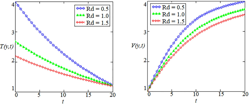
Fig. 2 is depicted to emphasize the effects of thermal radiation on temperature and velocity profiles. It is observed that profile of temperature is sequestrating while velocity field has scattering behavior of fluid flow over the boundary of plate. This is due to increase in thermal radiation which produces sequestrating and scattering behavior of fluid flow.
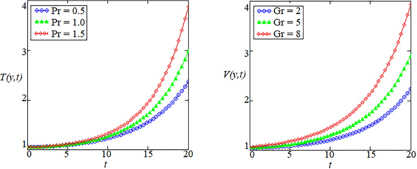
Fig. 3 is prepared to illustrate the influence on temperature field for viscous and thermal forces and velocity profile for buoyancy forces. It is noted that profiles of temperature and velocity field have quit identical behavior to each other while increase in Prandtl number $P_{r}$ and Grashof number $G_{r}$ respectively.
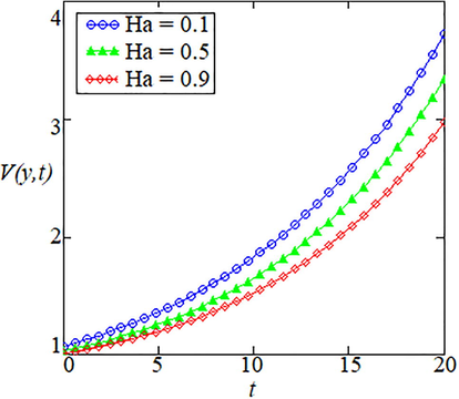
The effect of transverse magnetic field $M$ is highlighted in Fig. 4, in which pattern of oscillating is dominant in velocity distribution. Due to applied magnetic field, flow of velocity field is smattering and scattering with monotonic effect.
The Caputo–Fabrizio fractional parameter $ζ$ is emphasized in Fig. 5 to characterize memory properties on temperature distribution and velocity field. The effect of Caputo–Fabrizio fractional parameter $ζ$ seems to be identical qualitatively as expected for both temperature and velocity.
Fig. 6 is prepared for comparison of ordinary velocity field and fractionalized velocity field with four models i-e (i) Jeffery fluid with magnetic field (ii) Jeffery fluid without magnetic field (iii) Second grade fluid with magnetic field and (iv) Second grade fluid without magnetic field. It is worth pointing out that ordinary fluid is extremely sequestrating in contrast with fractionalized fluid. Ordinary Jeffery fluid with magnetic field oscillates more rapidly to remaining models of fluid but fractionalized Jeffery fluid with magnetic field has reciprocal behavior of fluid flow. The similar phenomenon can also be assessed for temperature distribution via graphical illustrations as well.

Effects of thermal radiation on temperature distribution and velocity field.

Effects of Prandtl and Grashof number on temperature distribution and velocity field.

Effects of Hartman number on the velocity field.

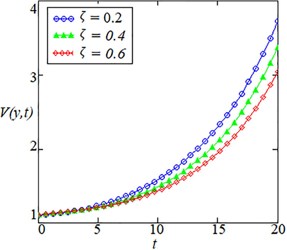
Effects of Caputo-Fabrizio fractional parameter on the velocity field.

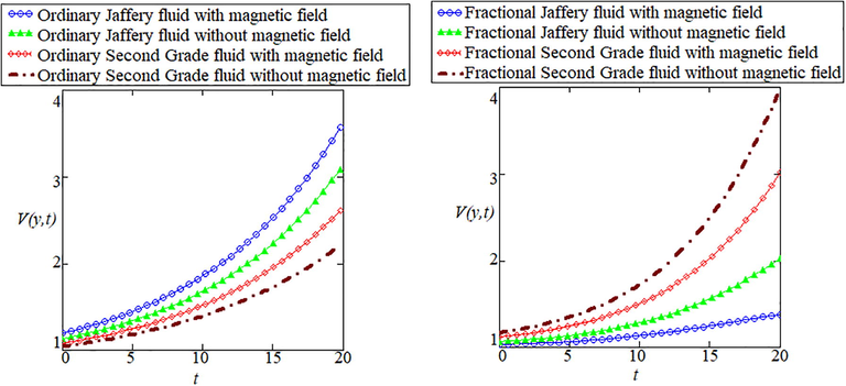
Comparison of Ordinary Jaffery and Second grade fluid with and without magnetic field on the velocity field.

References

Ver Strate G., Struglinski M.J., . Polymers as lubricating-oil viscosity modifiers. In: Polymers as Rheology Modifiers, Proceedings of the ACS Symposium Series. American Chemical Society; 1991. p. :256-272.
[Google Scholar]
Suryawanshi S.S., Kunjwani H.K., Kawade Jayashree V., Alkunte Mohita A., Yadav Dattatraya J., . J. Adv. Pharmaceut. Technol. Res.. 2012;2:67.
Balmforth N.J., Craster R.V., . J. Non-Newtonian Fluid Mech.. 1999;84:65.
Jokuty P., Fingas M., Whiticar S., Fieldhouse B., . A Study of Viscosity and Interfacial Tension of Oils and Emulsions. Ottawa, Ontario: Environment Canada Manuscript Report Number EE-153; 1995.
Tripathi D., Anwar Bég O., . Peristaltic propulsion of generalized Burgers’ fluids through a non-uniform porous medium: A study of chyme dynamics through the diseased intestine. Math. Biosci.. 2014;248:67-77.
[Google Scholar]
Sisko A.W., . The flow of lubricating greases. Ind. Eng. Chem.. 1958;50(12):1789-1792.
[Google Scholar]
Sahoo Bikash, Poncet Sebastien, . Flow and heat transfer of a third grade fluid past an exponentially stretching sheet with partial slip boundary condition. Int. J. Heat and Mass Trans., Elsevier. 2011;54:5010-5019.
[Google Scholar]
Sarpkaya T., Rainey P.G., . Stagnation point flow of a second-order viscoelastic fluid. Acta Mech.. 1971;11:237.
[Google Scholar]
Khan I., Fakhar K., Anwar M.I., . Hydromagnetic rotating flows of an Oldroyd-B fluid in a porous medium. Spec. Top. Rev. Porous Media. 2012;3:89-95.
[Google Scholar]
Abro Kashif Ali, Shaikh Asif Ali, Junejo Ishtiaque Ahmed, . Analytical Solutions Under No Slip Effects for Accelerated Flows of Maxwell Fluids, Sindh Univ. Res. Jour. (Sci. Ser.). 2015;47:613-618.
[Google Scholar]
Abro Kashif Ali, Shaikh Asif Ali, . Exact analytical solutions for Maxwell fluid over an oscillating plane. Sci. Int. (Lahore) ISSN.. 2015;27:923-929.
[Google Scholar]
Qasim M., . Heat and mass transfer in a Jeffrey fluid over a stretching sheet with heat source/sink. Alexandria Eng. J.. 2013;52:571-575.
[Google Scholar]
Hayat T., Mustafa M., . Influence of thermal radiation on the unsteady mixed convection flow of a Jeffrey fluid over a stretching sheet. Z. Naturforsch.. 2010;65:711-719.
[Google Scholar]
Nadeem S., Tahir B., Labropulu F., Akbar N.S., . Unsteady oscillatory stagnation point flow of a Jeffrey fluid. J. Aerosp. Eng.. 2014;27(3):636-643.
[Google Scholar]
Hayat T., Shehzad S.A., Qasim M., Obaidat S., . Radiative flow of Jeffery fluid in a porous medium with power law heat flux and heat source. Nucl. Eng. Des.. 2012;243:15-19.
[Google Scholar]
Shehzad S.A., Alsaedi A., Hayat T., . Influence of thermophoresis and joule heating on the radiative flow of Jeffrey fluid with mixed convection. Braz. J. Chem. Eng.. 2013;30(4):897-908.
[Google Scholar]
Khan I., . A note on exact solutions for the unsteady free convection flow of a jeffrey fluid. Z. Naturforschung A. 2015;70(6):272-284.
[Google Scholar]
Dalir N., . Numerical study of entropy generation for forced convection flow and heat transfer of a Jeffrey fluid over a stretching sheet. Alexandria Eng. J.. 2014;53(4):769-778.
[Google Scholar]
Hayat T., Khan M., Fakhar K., Amin N., . Oscillatory rotating flows of a fractional Jeffrey fluid filling a porous space. J. Porous Media. 2010;13(1):29-38.
[Google Scholar]
Idowu A.S., Joseph K.M., Daniel S., . Effect of heat and mass transfer on unsteady MHD oscillatory flow of Jeffrey fluid in a horizontal channel with chemical reaction. IOSR J. Math.. 2013;8(5):74-87.
[Google Scholar]
Abro Kashif Ali, Solangi Muhammad Anwar, . Heat transfer in magnetohydrodynamic second grade fluid with porous impacts using caputo-fabrizoi fractional derivatives. Punjab Univ. J. Math.. 2017;49(2):113-125.
[Google Scholar]
Sheikholeslami, Rokni Houman B., . Magnetic nanofluid flow and convective heat transfer in a porous cavity considering Brownian motion effects. Phys. Fluids. 2018;30:012003
[CrossRef] [Google Scholar]
Abro Kashif Ali, Hussain Mukarrum, Baig Mirza Mahmood, . A mathematical analysis of magnetohydrodynamic generalized burger fluid for permeable oscillating plate. Punjab Univ. J. Mathematics. 2018;50(2):97-111.
[Google Scholar]
Atangana Abdon, Koca Ilknur, . Chaos in a simple nonlinear system with Atangana-Baleanu derivatives with fractional order. Chaos, Solitons Fractals. 2016;89:447-454.
[Google Scholar]
Abro Kashif Ali, Hussain Mukarrum, Baig Mirza Mahmood, . An analytic study of molybdenum disulfide nanofluids using modern approach of atangana-baleanu fractional derivatives. Eur. Phys. J. Plus Eur. Phys. J. Plus. 2017;132:439.
[CrossRef] [Google Scholar]
Abro Kashif Ali, Chandio Ali Dad, Abro Irfan Ali, Khan Ilyas, . Dual thermal analysis of magnetohydrodynamic flow of nanofluids via modern approaches of Caputo-Fabrizio and Atangana-Baleanu fractional derivatives embedded in porous medium. J. Therm. Anal. Calorim. 2018:1-11.
[CrossRef] [Google Scholar]
Khan Ilyas, Abro Kashif Ali, . Thermal analysis in Stokes’ second problem of nanofluid: applications in thermal engineering. Case Stud. Thermal Eng.. 2018;10
[CrossRef] [Google Scholar]
Abro Kashif Ali, Hussain Mukarrum, Baig Mirza Mahmood, . Analytical solution of MHD generalized burger’s fluid embedded with porosity. Int. J. Adv. Appl. Sci.. 2017;4(7):80-89.
[Google Scholar]
Abro Kashif Ali, Solangi Muhammad Anwar, Laghari Muzaffar Hussain, . Influence of slippage in heat and mass transfer for fractionalized MHD flows in porous medium. Int. J. Adv. Appl. Math. Mech.. 2017;4(4):5-14.
[Google Scholar]
Atangana Abdon, . On the new fractional derivative and application to nonlinear Fisher's reaction-diffusion equation. Appl. Math. Comput.. 2016;273:948-956.
[Google Scholar]
Sheikholeslami M., Darzi Milad, Li Zhixiong, . Experimental investigation for entropy generation and exergy loss of nano-refrigerant condensation process. Int. J. Heat Mass Transf.. 2018;125:1087-1095.
[Google Scholar]
Abro Kashif Ali, Khan Ilyas, . Analysis of heat and mass transfer in MHD flow of generalized casson fluid in a porous space via non-integer order derivative without singular kernel. Chin. J. Phys.. 2017;55(4):1583-1595.
[Google Scholar]
Sheikholeslami M., Shehzad S.A., Abbasi F.M., Li Zhixiong, . Nanofluid flow and forced convection heat transfer due to Lorentz forces in a porous lid driven cubic enclosure with hot obstacle. Meth. Appl. Mech. Eng.. 2018;338:491-505.
[Google Scholar]
Abro Kashif Ali, Rashidi Mohammad Mehdi, Khan Ilyas, Abro Irfan Ali, Tassadiq Asifa, . Analysis of stokes’ second problem for nanofluids using modern fractional derivatives. J. Nanofluids. 2018;7:738-747.
[Google Scholar]
Mohyud-Din S.T., Zaidi Z.A., Khan U., Ahmed N., . On heat and mass transfer analysis for the flow of a nanofluid between rotating parallel plates. Aerosp. Sci. Technol.. 2015;46:514-522.
[Google Scholar]
Khan Arshad, Abro Kashif Ali, Tassaddiq Asifa, Khan Ilyas, . Atangana-baleanu and caputo fabrizio analysis of fractional derivatives for heat and mass transfer of second grade fluids over a vertical plate: a comparative study. Entropy. 2017;19(8):1-12.
[Google Scholar]
Sheikholeslami M., Shehzad S.A., Li Zhixiong, . Water based nanofluid free convection heat transfer in a three dimensional porous cavity with hot sphere obstacle in existence of Lorenz forces. Int. J. Heat Mass Transf.. 2018;125:375-386.
[Google Scholar]
Sheikholeslami M., Darzi Milad, Sadoughi M.K., . Heat transfer improvement and pressure drop during condensation of refrigerant-based nanofluid; an experimental procedure. Int. J. Heat Mass Transf.. 2018;122:643-650.
[Google Scholar]
Khan U., Adnan, Ahmed N., Mohyud-Din S.T., . Heat transfer enhancement in hydromagnetic dissipative flow past a moving wedge suspended by H2O-aluminum alloy nanoparticles in the presence of thermal radiation. Int. J. Hydrogen Energy. 2017;42:24634-24644.
[Google Scholar]
Al-Mdallal Qasem, Abro Kashif Ali, Khan Ilyas, . Analytical solutions of fractional Walter’s-B fluid with applications. Complexity 2018 Article ID 8918541
[Google Scholar]
Saad Badr, Alkahtani T., Atangana A., . Generalized groundwater plume with degradation and rate-limited sorption model with Mittag-Leffler law. Res. Physics. 2017;7:4398-4404.
[Google Scholar]
Abro Kashif Ali, Memon Anwar Ahmed, Uqaili Muhammad Aslam, . A comparative mathematical analysis of RL and RC electrical circuits via Atangana-Baleanu and Caputo-Fabrizio fractional derivatives. Eur. Phys. J. Plus. 2018;133:113.
[CrossRef] [Google Scholar]
Atangana Abdon, Baleanu Dumitru, . Caputo-Fabrizio derivative applied to groundwater flow within confined aquifer. J. Eng. Mech.. 2017;143(5):D4016005.
[Google Scholar]
Laghari Muzaffar Hussain, Abro Kashif Ali, Shaikh Asif Ali, . Helical flows of fractional viscoelastic fluid in a circular pipe. Int. J. Adv. Appl. Sci.. 2017;4(10):97-105.
[Google Scholar]
Caputo M., Fabrizio M., . A new definition of fractional derivative without singular kernel. Progr. Fract. Differ. Appl.. 2015;1(2):73-85.
[Google Scholar]
Shah N.A., Khan I., . Heat transfer analysis in a second grade fluid over and oscillating vertical plate using fractional Caputo–Fabrizio derivatives. Eur. Phys. J. C 2016:362-376.
[Google Scholar]
Zafar A.A., Fetecau C., . Flow over an infinite plate of a viscous fluid with non-integer order derivative without singular kernel. Alexandria Eng. J.. 2016;55(3):2789-2796.
[Google Scholar]
Abro Kashif Ali, Shaikh Asif Ali, Dehraj Sanuallah, . Exact solutions on the oscillating plate of maxwell fluids. Mehran Univ. Res. J. Eng. Technol.. 2016;35(1):157-162.
[Google Scholar]
Abro Kashif Ali, . Porous effects on second grade fluid in oscillating plate. J. Appl. Environ. Biol. Sci.. 2016;6:71-82.
[Google Scholar]
Samiulhaq I., Khan F. Ali, Shafie S., . Free, convection flow of a second-grade fluid with ramped wall temperature. Heat Trans. Res.. 2014;45(7):579-588.
[Google Scholar]
Zin Nor Athirah Mohd, Khan Ilyas, Shafie Sharidan, . Influence of thermal radiation on unsteady MHD free convection flow of Jeffrey fluid over a vertical plate with ramped wall temperature. Math. Prob. Eng. 2016
[CrossRef] [Google Scholar]

Introduction

Governing equations

Profile of temperature distribution via Fourier Sine transform

Profile of velocity field via Fourier Sine transform

Limiting cases

Temperature distribution and velocity field without the effects of radiation when Rd = 0
Velocity field without the effects of magnetic field when H a = 0 .
Velocity field for Second grade fluid with magnetic field when λ 1 = 0 and H a ≠ 0 .

Discussions and concluding remarks

Fulltext Views
33

PDF downloads
23

View/Download PDF
Download Citations

BibTeX
RIS

Show Sections

[1] Ver Strate G., Struglinski M.J., . Polymers as lubricating-oil viscosity modifiers. In: Polymers as Rheology Modifiers, Proceedings of the ACS Symposium Series. American Chemical Society; 1991. p. :256-272.
[Google Scholar]

[2] Suryawanshi S.S., Kunjwani H.K., Kawade Jayashree V., Alkunte Mohita A., Yadav Dattatraya J., . J. Adv. Pharmaceut. Technol. Res.. 2012;2:67.

[3] Balmforth N.J., Craster R.V., . J. Non-Newtonian Fluid Mech.. 1999;84:65.

[4] Jokuty P., Fingas M., Whiticar S., Fieldhouse B., . A Study of Viscosity and Interfacial Tension of Oils and Emulsions. Ottawa, Ontario: Environment Canada Manuscript Report Number EE-153; 1995.

[5] Tripathi D., Anwar Bég O., . Peristaltic propulsion of generalized Burgers’ fluids through a non-uniform porous medium: A study of chyme dynamics through the diseased intestine. Math. Biosci.. 2014;248:67-77.
[Google Scholar]

[6] Sisko A.W., . The flow of lubricating greases. Ind. Eng. Chem.. 1958;50(12):1789-1792.
[Google Scholar]

[7] Sahoo Bikash, Poncet Sebastien, . Flow and heat transfer of a third grade fluid past an exponentially stretching sheet with partial slip boundary condition. Int. J. Heat and Mass Trans., Elsevier. 2011;54:5010-5019.
[Google Scholar]

[8] Sarpkaya T., Rainey P.G., . Stagnation point flow of a second-order viscoelastic fluid. Acta Mech.. 1971;11:237.
[Google Scholar]

[9] Khan I., Fakhar K., Anwar M.I., . Hydromagnetic rotating flows of an Oldroyd-B fluid in a porous medium. Spec. Top. Rev. Porous Media. 2012;3:89-95.
[Google Scholar]

[10] Abro Kashif Ali, Shaikh Asif Ali, Junejo Ishtiaque Ahmed, . Analytical Solutions Under No Slip Effects for Accelerated Flows of Maxwell Fluids, Sindh Univ. Res. Jour. (Sci. Ser.). 2015;47:613-618.
[Google Scholar]

[11] Abro Kashif Ali, Shaikh Asif Ali, . Exact analytical solutions for Maxwell fluid over an oscillating plane. Sci. Int. (Lahore) ISSN.. 2015;27:923-929.
[Google Scholar]

[12] Qasim M., . Heat and mass transfer in a Jeffrey fluid over a stretching sheet with heat source/sink. Alexandria Eng. J.. 2013;52:571-575.
[Google Scholar]

[13] Hayat T., Mustafa M., . Influence of thermal radiation on the unsteady mixed convection flow of a Jeffrey fluid over a stretching sheet. Z. Naturforsch.. 2010;65:711-719.
[Google Scholar]

[14] Nadeem S., Tahir B., Labropulu F., Akbar N.S., . Unsteady oscillatory stagnation point flow of a Jeffrey fluid. J. Aerosp. Eng.. 2014;27(3):636-643.
[Google Scholar]

[15] Hayat T., Shehzad S.A., Qasim M., Obaidat S., . Radiative flow of Jeffery fluid in a porous medium with power law heat flux and heat source. Nucl. Eng. Des.. 2012;243:15-19.
[Google Scholar]

[16] Shehzad S.A., Alsaedi A., Hayat T., . Influence of thermophoresis and joule heating on the radiative flow of Jeffrey fluid with mixed convection. Braz. J. Chem. Eng.. 2013;30(4):897-908.
[Google Scholar]

[17] Khan I., . A note on exact solutions for the unsteady free convection flow of a jeffrey fluid. Z. Naturforschung A. 2015;70(6):272-284.
[Google Scholar]

[18] Dalir N., . Numerical study of entropy generation for forced convection flow and heat transfer of a Jeffrey fluid over a stretching sheet. Alexandria Eng. J.. 2014;53(4):769-778.
[Google Scholar]

[19] Hayat T., Khan M., Fakhar K., Amin N., . Oscillatory rotating flows of a fractional Jeffrey fluid filling a porous space. J. Porous Media. 2010;13(1):29-38.
[Google Scholar]

[20] Idowu A.S., Joseph K.M., Daniel S., . Effect of heat and mass transfer on unsteady MHD oscillatory flow of Jeffrey fluid in a horizontal channel with chemical reaction. IOSR J. Math.. 2013;8(5):74-87.
[Google Scholar]

[21] Abro Kashif Ali, Solangi Muhammad Anwar, . Heat transfer in magnetohydrodynamic second grade fluid with porous impacts using caputo-fabrizoi fractional derivatives. Punjab Univ. J. Math.. 2017;49(2):113-125.
[Google Scholar]

[22] Sheikholeslami, Rokni Houman B., . Magnetic nanofluid flow and convective heat transfer in a porous cavity considering Brownian motion effects. Phys. Fluids. 2018;30:012003
[CrossRef] [Google Scholar]

[23] Abro Kashif Ali, Hussain Mukarrum, Baig Mirza Mahmood, . A mathematical analysis of magnetohydrodynamic generalized burger fluid for permeable oscillating plate. Punjab Univ. J. Mathematics. 2018;50(2):97-111.
[Google Scholar]

[24] Atangana Abdon, Koca Ilknur, . Chaos in a simple nonlinear system with Atangana-Baleanu derivatives with fractional order. Chaos, Solitons Fractals. 2016;89:447-454.
[Google Scholar]

[25] Abro Kashif Ali, Hussain Mukarrum, Baig Mirza Mahmood, . An analytic study of molybdenum disulfide nanofluids using modern approach of atangana-baleanu fractional derivatives. Eur. Phys. J. Plus Eur. Phys. J. Plus. 2017;132:439.
[CrossRef] [Google Scholar]

[26] Abro Kashif Ali, Chandio Ali Dad, Abro Irfan Ali, Khan Ilyas, . Dual thermal analysis of magnetohydrodynamic flow of nanofluids via modern approaches of Caputo-Fabrizio and Atangana-Baleanu fractional derivatives embedded in porous medium. J. Therm. Anal. Calorim. 2018:1-11.
[CrossRef] [Google Scholar]

[27] Khan Ilyas, Abro Kashif Ali, . Thermal analysis in Stokes’ second problem of nanofluid: applications in thermal engineering. Case Stud. Thermal Eng.. 2018;10
[CrossRef] [Google Scholar]

[28] Abro Kashif Ali, Hussain Mukarrum, Baig Mirza Mahmood, . Analytical solution of MHD generalized burger’s fluid embedded with porosity. Int. J. Adv. Appl. Sci.. 2017;4(7):80-89.
[Google Scholar]

[29] Abro Kashif Ali, Solangi Muhammad Anwar, Laghari Muzaffar Hussain, . Influence of slippage in heat and mass transfer for fractionalized MHD flows in porous medium. Int. J. Adv. Appl. Math. Mech.. 2017;4(4):5-14.
[Google Scholar]

[30] Atangana Abdon, . On the new fractional derivative and application to nonlinear Fisher's reaction-diffusion equation. Appl. Math. Comput.. 2016;273:948-956.
[Google Scholar]

[31] Sheikholeslami M., Darzi Milad, Li Zhixiong, . Experimental investigation for entropy generation and exergy loss of nano-refrigerant condensation process. Int. J. Heat Mass Transf.. 2018;125:1087-1095.
[Google Scholar]

[32] Abro Kashif Ali, Khan Ilyas, . Analysis of heat and mass transfer in MHD flow of generalized casson fluid in a porous space via non-integer order derivative without singular kernel. Chin. J. Phys.. 2017;55(4):1583-1595.
[Google Scholar]

[33] Sheikholeslami M., Shehzad S.A., Abbasi F.M., Li Zhixiong, . Nanofluid flow and forced convection heat transfer due to Lorentz forces in a porous lid driven cubic enclosure with hot obstacle. Meth. Appl. Mech. Eng.. 2018;338:491-505.
[Google Scholar]

[34] Abro Kashif Ali, Rashidi Mohammad Mehdi, Khan Ilyas, Abro Irfan Ali, Tassadiq Asifa, . Analysis of stokes’ second problem for nanofluids using modern fractional derivatives. J. Nanofluids. 2018;7:738-747.
[Google Scholar]

[35] Mohyud-Din S.T., Zaidi Z.A., Khan U., Ahmed N., . On heat and mass transfer analysis for the flow of a nanofluid between rotating parallel plates. Aerosp. Sci. Technol.. 2015;46:514-522.
[Google Scholar]

[36] Khan Arshad, Abro Kashif Ali, Tassaddiq Asifa, Khan Ilyas, . Atangana-baleanu and caputo fabrizio analysis of fractional derivatives for heat and mass transfer of second grade fluids over a vertical plate: a comparative study. Entropy. 2017;19(8):1-12.
[Google Scholar]

[37] Sheikholeslami M., Shehzad S.A., Li Zhixiong, . Water based nanofluid free convection heat transfer in a three dimensional porous cavity with hot sphere obstacle in existence of Lorenz forces. Int. J. Heat Mass Transf.. 2018;125:375-386.
[Google Scholar]

[38] Sheikholeslami M., Darzi Milad, Sadoughi M.K., . Heat transfer improvement and pressure drop during condensation of refrigerant-based nanofluid; an experimental procedure. Int. J. Heat Mass Transf.. 2018;122:643-650.
[Google Scholar]

[39] Khan U., Adnan, Ahmed N., Mohyud-Din S.T., . Heat transfer enhancement in hydromagnetic dissipative flow past a moving wedge suspended by H2O-aluminum alloy nanoparticles in the presence of thermal radiation. Int. J. Hydrogen Energy. 2017;42:24634-24644.
[Google Scholar]

[40] Al-Mdallal Qasem, Abro Kashif Ali, Khan Ilyas, . Analytical solutions of fractional Walter’s-B fluid with applications. Complexity 2018 Article ID 8918541
[Google Scholar]

[41] Saad Badr, Alkahtani T., Atangana A., . Generalized groundwater plume with degradation and rate-limited sorption model with Mittag-Leffler law. Res. Physics. 2017;7:4398-4404.
[Google Scholar]

[42] Abro Kashif Ali, Memon Anwar Ahmed, Uqaili Muhammad Aslam, . A comparative mathematical analysis of RL and RC electrical circuits via Atangana-Baleanu and Caputo-Fabrizio fractional derivatives. Eur. Phys. J. Plus. 2018;133:113.
[CrossRef] [Google Scholar]

[43] Atangana Abdon, Baleanu Dumitru, . Caputo-Fabrizio derivative applied to groundwater flow within confined aquifer. J. Eng. Mech.. 2017;143(5):D4016005.
[Google Scholar]

[44] Laghari Muzaffar Hussain, Abro Kashif Ali, Shaikh Asif Ali, . Helical flows of fractional viscoelastic fluid in a circular pipe. Int. J. Adv. Appl. Sci.. 2017;4(10):97-105.
[Google Scholar]

[45] Caputo M., Fabrizio M., . A new definition of fractional derivative without singular kernel. Progr. Fract. Differ. Appl.. 2015;1(2):73-85.
[Google Scholar]

[46] Shah N.A., Khan I., . Heat transfer analysis in a second grade fluid over and oscillating vertical plate using fractional Caputo–Fabrizio derivatives. Eur. Phys. J. C 2016:362-376.
[Google Scholar]

[47] Zafar A.A., Fetecau C., . Flow over an infinite plate of a viscous fluid with non-integer order derivative without singular kernel. Alexandria Eng. J.. 2016;55(3):2789-2796.
[Google Scholar]

[48] Abro Kashif Ali, Shaikh Asif Ali, Dehraj Sanuallah, . Exact solutions on the oscillating plate of maxwell fluids. Mehran Univ. Res. J. Eng. Technol.. 2016;35(1):157-162.
[Google Scholar]

[49] Abro Kashif Ali, . Porous effects on second grade fluid in oscillating plate. J. Appl. Environ. Biol. Sci.. 2016;6:71-82.
[Google Scholar]

[50] Samiulhaq I., Khan F. Ali, Shafie S., . Free, convection flow of a second-grade fluid with ramped wall temperature. Heat Trans. Res.. 2014;45(7):579-588.
[Google Scholar]

[51] Zin Nor Athirah Mohd, Khan Ilyas, Shafie Sharidan, . Influence of thermal radiation on unsteady MHD free convection flow of Jeffrey fluid over a vertical plate with ramped wall temperature. Math. Prob. Eng. 2016
[CrossRef] [Google Scholar]

On the thermal analysis of magnetohydrodynamic Jeffery fluid via modern non integer order derivative

Abstract

Keywords

Thermal radiation

Jeffery fluid

Caputo-Fabrizio fractional derivative

Fourier Sine and Laplace transform

1 Introduction

2 Governing equations

3 Profile of temperature distribution via Fourier Sine transform

4 Profile of velocity field via Fourier Sine transform

5 Limiting cases

5.1 Temperature distribution and velocity field without the effects of radiation when Rd = 0

5.2 Velocity field without the effects of magnetic field when H a = 0 .

5.3 Velocity field for Second grade fluid with magnetic field when λ 1 = 0 and H a ≠ 0 .

6 Discussions and concluding remarks

References

Suggested read for related articles:

5.1 Temperature distribution and velocity field without the effects of radiation when $Rd = 0$

5.2 Velocity field without the effects of magnetic field when $H_{a} = 0 .$

5.3 Velocity field for Second grade fluid with magnetic field when $λ_{1} = 0$ and $H_{a} \neq 0 .$