Logarithmic inverse Lindley distribution: Model, properties and applications

1 Introduction

“The Lindley distribution was proposed by Lindley (1958) in the context of the Bayes theorem as a counter example of fiducial statistics with the probability density function (pdf)”

“Ghitany et al. (2008) discussed the Lindley distribution and its applications extensively and showed that the Lindley distribution is a better fit than the exponential distribution based on the waiting time at the bank for service.”

“Mazucheli and Achcar (2011) worked on the Lindley distribution applied to competing risks lifetime data. Krishna and Kumar (2011) estimated the parameter of Lindley distribution with progressive Type-II censoring scheme. They also showed that it may be better lifetime model than exponential, lognormal and gamma distributions in some real life situations. Since then the distribution has been widely discussed in various context. Singh and Gupta (2012) have used the Lindley distribution under load sharing system models. Al-Mutairi et al. (2013) developed the inferential procedure of the stress-strength parameter, when both stress and strength variables follow Lindley distribution. It may be mentioned here that the Lindley distribution is useful when the data show increasing failure rate. This is the property that encourage the use of Lindley distribution in lifetime data analysis over exponential distribution. Although the family of Lindley distributions possess very nice properties and gained great applicability in various disciplines, its applicability may be restricted to non-monotone upside down bathtub (UBT) hazard rate data see Sharma et al. (2014). Therefore, the Lindley distribution has been extended to various ageing classes and introduced various generalized class of lifetime distribution based on Lindley distribution. Zakerzadeh and Dolati (2009) introduced three parameters extension of the Lindley distribution. Nadarajah et al. (2011), Ghitany et al. (2013) proposed two parameter generalizations of the Lindley distribution, called as the generalized Lindley and power Lindley distributions. These distributions are generated using the exponentiation and power transformations to the Lindley distribution. Merovci (2013) and Merovci and Elbatal (2014) investigated transmuted Lindley and transmuted Lindley-geometric distributions respectively. The beta-Lindley distribution is introduced by Merovci and Sharma (2014). Statistical and mathematical properties of Kumaraswamy Quasi Lindley and Kumaraswamy Lindley distributions are discussed by Elbatal and Elgarhy (2013) and Akmakyapan and Kadlar (2014) respectively. The exponentiated power Lindley distribution is introduced by Ashour and Eltehiwy (2015). The generalized Poisson-Lindley and another extension of the Lindley distribution are discussed by Mahmoudi and Zakerzadeh (2010) and Oluyede and Yang (2015)”.

“Shanker and Mishra (2013) proposed two parameter extensions of the Lindley distribution with the pdf” $$f(z\text{,}\theta )=\frac{{\theta }^2}{\beta +\theta }(1+\beta z)e^{-\theta z}\text{;}z>0\text{,}\theta \text{,}\beta >0$$

In the references cited above, authors mainly focused on the estimation of increasing, decreasing and bathtub shaped failure rates data. Nobody has paid attention to the modelling of the upside down bathtub data. “Recently, the inverse Lindley distribution was introduced by Sharma et al. (2015) using the transformation $X=\frac{1}{T}$ with density and cumulative distribution functions defined, respectively, by”:

and

where T is a random variable having pdf (1).

“Sharma et al. (2015) discussed the properties of inverse Lindley distribution with application to stress strength reliability analysis. Sharma et al. (2016) introduced two parameter extension of inverse Lindley distribution using power transformation to inverse Lindley random variable. Recently, Alkarni (2015) proposed three parameter inverse Lindley distribution with application to maximum flood level data”.

“Another two parameter inverse Lindley distribution introduced by Barco et al. (2017), called “the power inverse Lindley distribution,” is a new statistical inverse model for upside-down bathtub survival data that uses the transformation $X=T^{-\frac{1}{\alpha }}$ with the following pdf ”, $$f(x\text{,}\theta \text{,}\alpha )=\frac{\alpha {\theta }^2}{1+\theta }\left(\frac{1+x^{\alpha }}{x^{2\alpha +1}}\right)e^{-\frac{\theta }{x^{\alpha }}}\text{;}\theta \text{,}\alpha \text{,}x>0$$

In this paper, we proposed another extension of inverse Lindley distribution which offers more flexibility with an effective shape parameter. To this end, an extension of the Marshall-Olkin generalization approach, by Marshall and Olkin (1997), has been used. This generalization method introduced by Pappas et al. (2012). We refer to the new model as the Logarithmic inverse Lindley (LIL) distribution.

“Pappas et al. (2012) proposed a generalization formula of a distribution G(x) that introduces a new parameter $\beta >0$ ”. This approach is defined through the cumulative distribution function (cdf).

where $\overline{G}(x)=1-G(x)$ is the survival (or reliability) function of the inverse Lindley distribution.

Now, combining Eqs. (3) and (4) and simplifying the expression leads to the cdf of the Logarithmic-inverse Lindley distribution as

By differentiating Eq. (5) with respect to x, then the pdf after some simplifications can be written as

For $\beta \in (0\text{,}1)$ , the pdf given by Eq. (6) can be obtained as a compound of the Logarithmic and the inverse Lindley distributions. “According to Barlow and Proschan (1996) and Arnold et al. (1992), consider the lifetime $X=\text{min}(X_1\text{,}{X}_1\text{,}\dots \text{,}{X}_N)$ of a series system of $N$ identical components. If the lifetimes of the components are iid random variables with survivals given by (2) and the distribution of their number $n$ is Logarithmic, independently of the X’s, with pmf

and the conditional pdf of $(X/N=n)$ is given by

Then, the joint distribution of the random variables $X$ and $N$ , denoted by $f(x\text{,}n)$ , is obtained as $$f(x\text{,}n)=f(x|n).P(N=n)=\frac{-{(1-\beta )}^n{\theta }^2(1+x)e^{-\frac{\theta }{x}}}{(1+\theta )x^3\ln \beta }{\left[(1-\beta )\left(1-\left(1+\frac{\theta }{(1+\theta )x}\right)e^{-\frac{\theta }{x}}\right)\right]}^{n-1}$$

Hence, it can be found the marginal pdf of $X$ follows

Tahmasbi and Rezaei (2008), proposed the exponential-logarithmic distribution using the same procedure. Warahena-Liyanage and Pararai (2015) proposed the logarithmic Lindley distribution and studied its properties as special case of The Lindley Power series class of Distributions.

The following propositions discuss the limiting behavior and other characteristics of LIL distribution.

Proposition 1. The inverse Lindley is a limiting distribution of the LIL distribution when $\beta \to 1$ .

Proof. Using Eq. (5) $${\lim }_{\beta \to 1}F(x\text{,}\theta \text{,}\beta )=1-{\lim }_{\beta \to 1}\frac{\ln \left[1-(1-\beta )\left(1-\left(1+\frac{\theta }{(1+\theta )x}\right)e^{-\frac{\theta }{x}}\right)\right]}{\ln \beta }$$

By using L'Hopital’s rule, we obtain $${\displaystyle \underset{\beta \to 1}{\lim }}F(x\text{,}\theta \text{,}\beta )=1-{\displaystyle \underset{\beta \to 1}{\lim }}\frac{\beta \left(1-\left(1+\frac{\theta }{(1+\theta )x}\right)e^{-\frac{\theta }{x}}\right)}{\left[1-(1-\beta )\left(1-\left(1+\frac{\theta }{(1+\theta )x}\right)e^{-\frac{\theta }{x}}\right)\right]}=\left(1+\frac{\theta }{(1+\theta )x}\right)e^{-\frac{\theta }{x}}$$

Clearly, for $\beta \to 1$ ; the proposed model (LIL distribution) given in Eq. (6) reduces to the inverse Lindley distribution. Therefore, the LIL distribution can be viewed as an extension of the base model (which is asymptotically related to the usual one-parameter inverse Lindley distribution).

Proposition 2. For the pdf of the LIL distribution, we have $${\displaystyle \underset{x\to 0}{\lim }}f(x\text{,}\theta \text{,}\beta )=0$$

and $${\displaystyle \underset{x\to {\infty }^{+}}{\lim }}f(x\text{,}\theta \text{,}\beta )=0$$

The LIL distribution is always unimodal. Fig. 1 illustrates some of the possible shapes of the pdf of the LIL distribution for different values of the parameters $\theta$ and $\beta$ .

Close

Fig. 1

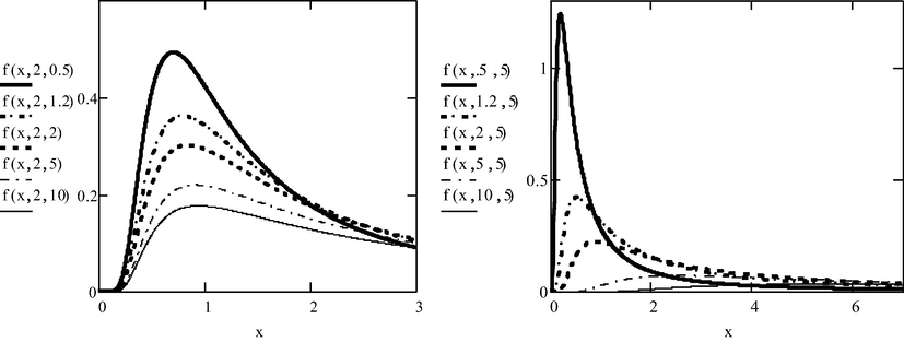
Probability density function of the LIL distribution for $\theta =2$ and $\beta =(0.5\text{,}1.2\text{,}2\text{,}5\text{,}10)$ (left); for $\theta =(0.5\text{,}1.2\text{,}2\text{,}5\text{,}10)$ and $\beta =5$ (right).

Export to PPT

Plots of the pdf are shown in Fig. 1. The pdfs appear always unimodal. The mode moves more to the right and the pdf becomes less peaked with increasing values of $\beta$ . The mode moves more to the right and the pdf becomes less peaked with increasing values of $\theta$ .

2 Reliability analysis

In this section, we present the survival (or reliability) function and study the hazard (or failure) rate function. Also, the cumulative hazard rate function and the mean residual lifetime are obtained for the LIL distribution.

2.1

2.1 The survival and hazard rate function

The survival function of the LIL distribution, denoted by R(x), is given by $$R(x)=1-F(x)=\frac{\ln \left[1-(1-\beta )\left(1-\left(1+\frac{\theta }{(1+\theta )x}\right)e^{-\frac{\theta }{x}}\right)\right]}{\ln \beta }$$

The other characteristic of interest of a random variable is the hazard rate function, h(x), also known as instantaneous failure rate which is an important quantity characterizing life phenomenon. The hazard rate function for a LIL distribution is given by

(11)

$$h(x)=\frac{f(x)}{R(x)}=\frac{\frac{(\beta -1){\theta }^2}{1+\theta }\left(\frac{1+x}{x^3}\right)e^{-\frac{\theta }{x}}}{\left[1-(1-\beta )\left(1-\left(1+\frac{\theta }{(1+\theta )x}\right)e^{-\frac{\theta }{x}}\right)\right]\ln \left[1-(1-\beta )\left(1-\left(1+\frac{\theta }{(1+\theta )x}\right)e^{-\frac{\theta }{x}}\right)\right]}$$

Now, we shall study the behavior of the hazard rate function of the Log-IL distribution show its different shapes.

First, depending on Eqs. (2) and (3) we can compute the hazard rate function of the inverse Lindley distribution, denoted by $\eta (x)$ , as follows $$\eta (x)=\frac{\text{g}(x)}{1-\text{G}(x)}=\frac{{\theta }^2(1+x)}{x^2\left[\theta +x(1+\theta )\left(e^{-\frac{\theta }{x}}-1\right)\right]}$$

Then, by taking the limit of Eq. (11) when $x\to 0$ and when $x\to \infty$ as follows $${\lim }_{x\to 0}h(x)=\frac{\beta -1}{\beta \ln \beta }{\lim }_{x\to 0}\eta (x)=0\text{,}$$

and $${\lim }_{x\to \infty }h(x)={\lim }_{x\to \infty }\eta (x)=0$$

Because the hazard rate function of inverse Lindley distribution is always unimodel function in x, the new distribution is also a unimodal.

Fig. 2 illustrates the behavior of the hazard rate function of the LIL distribution at different values of the parameters involved.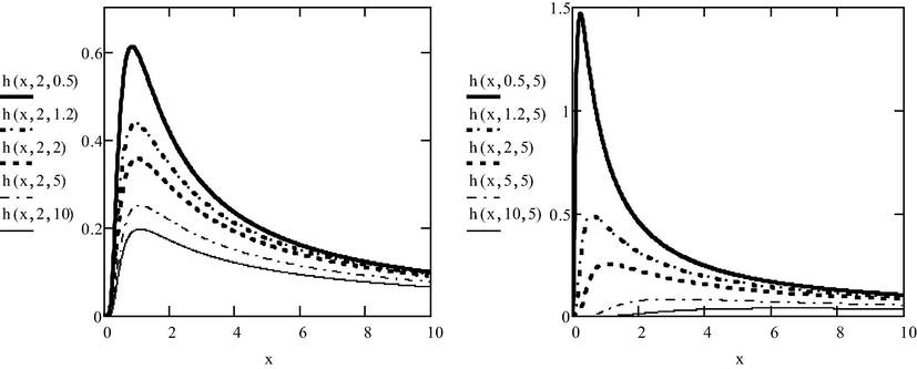

Close

Fig. 2

Hazard rate function of the LIL distribution for $\theta =2$ and $\beta =(0.5\text{,}1.2\text{,}2\text{,}5\text{,}10)$ (left); for $\theta =(0.5\text{,}1.2\text{,}2\text{,}5\text{,}10)$ and $\beta =5$ (right).

Export to PPT

Plots of the hazard rate function are shown in Fig. 2 indicates that the hazard function is upside down bathtub shaped. The hazard rate function appears always unimodal. Its shape becomes less peaked with increasing values of $\beta$ and less peaked with increasing values of $\theta$ .

3 Statistical properties

This section investigates the statistical properties of the LIL distribution such as the moments, the moment generating function, the quantiles and the median.

4 Estimation of the parameters

Let $x_1\text{,}\dots \text{,}{x}_n$ be a random sample of size n from LIL. Then, the log-likelihood function is given by

The MLEs $\widehat{\theta }\text{,}\widehat{\beta }$ of $\theta \text{,}\beta \text{,}$ are then the solutions of the following non-linear equations:

In order to solve above equations, one can apply a suitable iterative procedure such as the Newton- Raphson method.

5 Generation algorithms and Monte Carlo simulation study

In this section, the algorithms for generating random data from LIL distribution are given. A simulation study was also conducted to check the performance and accuracy of maximum likelihood estimates of the LIL model parameters.

6 Data analysis

In this section, we present example to illustrate the flexibility and superiority of the LIL distribution in modeling real data. We use a set of real data (given in Table 2) of flood levels to demonstrate the applicability of the LIL distribution. The data were obtained in a civil engineering context and gives the maximum flood level (in millions of cubic feet per second) for the Susquehanna River at Harrisburg, Pennsylvania over 20 four-year periods from 1890 to 1969. These data have been widely discussed by many authors and were initially reported by Dumonceaux and Antle (1973).We fit the density functions of LIL distribution in Eq. (6) and its sub-model the inverse Lindley (IL) distribution in Eq. (2).

We also compare the LIL distribution with seven alternative distributions such as:

• The inverse Weibull $(\mathit{IW}(\beta \text{,}\theta ))$ distribution specified by the pdf

• The inverse gamma $(\mathit{IGM}(\beta \text{,}\theta ))$ distribution specified by the pdf

The generalized inverse exponential $(\mathit{GIE}(\beta \text{,}\theta ))$ distribution specified by the pdf $$f(x)=\frac{\theta \beta }{x^2}{e}^{\frac{-\theta }{x}}{\left(1-e^{\frac{-\theta }{x}}\right)}^{\beta }\text{,}x\text{,}\beta \text{,}\theta >0$$

The inverse Gaussian $(\mathit{IG}(\beta \text{,}\theta ))$ distribution specified by the pdf $$f(x)={\left(\frac{\beta }{2\pi x^3}\right)}^{1/2}\mathit{exp}\left\{\frac{-\beta {(x-\theta )}^2}{2{\theta }^{2}x}\right\}\text{,}x\text{,}\beta \text{,}\theta >0$$

The lognormal $(\mathit{LN}(\mu \text{,}{\sigma }^2))$ distribution specified by the pdf $$f(x)=\frac{1}{\sqrt{2\pi }\sigma x}\mathit{exp}\left\{-\frac{{(\log x-\mu )}^2}{2{\sigma }^2}\right\}\text{,}x\text{,}\sigma >0\text{,}-\infty <\mu <\infty$$

The log-Logistic $(\mathit{LLog}(\beta \text{,}\theta ))$ distribution specified by the pdf $$f(x)=\frac{\beta }{\theta }{\left(\frac{x}{\theta }\right)}^{\beta -1}{\left(1+{\left(\frac{x}{\theta }\right)}^{\beta }\right)}^{-2}\text{,}x\text{,}\beta \text{,}\theta >0$$

The flexible Weibull $(\mathit{FW}(\beta \text{,}\theta ))$ distribution specified by the pdf $$f(x)=\left(\theta +\frac{\beta }{x^2}\right)e^{-\theta x-\frac{\beta }{x}}\mathit{exp}\left\{-e^{-\theta x-\frac{\beta }{x}}\right\}\text{,}x\text{,}\beta \text{,}\theta >0$$

For the data set, the estimates of the parameters of the distributions, Akaike information criterion (AIC) and Bayesian information criterion (BIC) are obtained. To choose the best possible model for the data set among all competitive models, the statistical tools used are described as follows: $\mathit{AIC}=-2\log L+2q$ and $\mathit{BIC}=-2\log L+q\log n$ , where, $q$ is the number of parameters are to be estimated from the data. Moreover, we apply the formal goodness of fit tests in order to verify which distribution fits better to these data. We consider the Cramer-von Mises $(W^{\ast })$ and Andrson-Darling $(A^{\ast })$ statistics. The statistics $W^{\ast }$ and $A^{\ast }$ are described in detail in Chen and Balakrishnan (1995). The statistic of the Kolmogorov-Smirnov test (KS as well as its respective p value is presented. This test observes the differences between the assumed cumulative distribution function and the empirical cumulative distribution function from the data to verify the fit of the distributions (p-value > 0.05). The sum of squares (SS) from the probability plots are also presented.

When comparing models, the model with the smallest AIC is considered to be the best fit model for a given data set. When selecting the best model for a given data set based on the values of SS, the model with the smallest SS is considered as the best fit model.

Fig. 3 shows the probability-probability (P-P) plot for all the fitted models. For the probability plot, we plotted $F_{\mathit{LogIL}}(x_{(j)}\text{;}\widehat{\beta }\text{,}\widehat{\theta })$ against $\frac{j-0.375}{n+0.25}\text{,}j=1\text{,}2\text{,}\dots \text{,}n$ , where $x_{(j)}$ are the ordered values of the observed data. The measures of closeness are given by the sum of squares $$\mathit{SS}={\displaystyle \sum _{j=1}^n}{\left[F_{\mathit{LogIL}}\left(x_{(j)}\text{;}\widehat{\beta }\text{,}\widehat{\theta }\right)-\frac{j-0.375}{n+0.25}\right]}^2$$

Close

Fig. 3

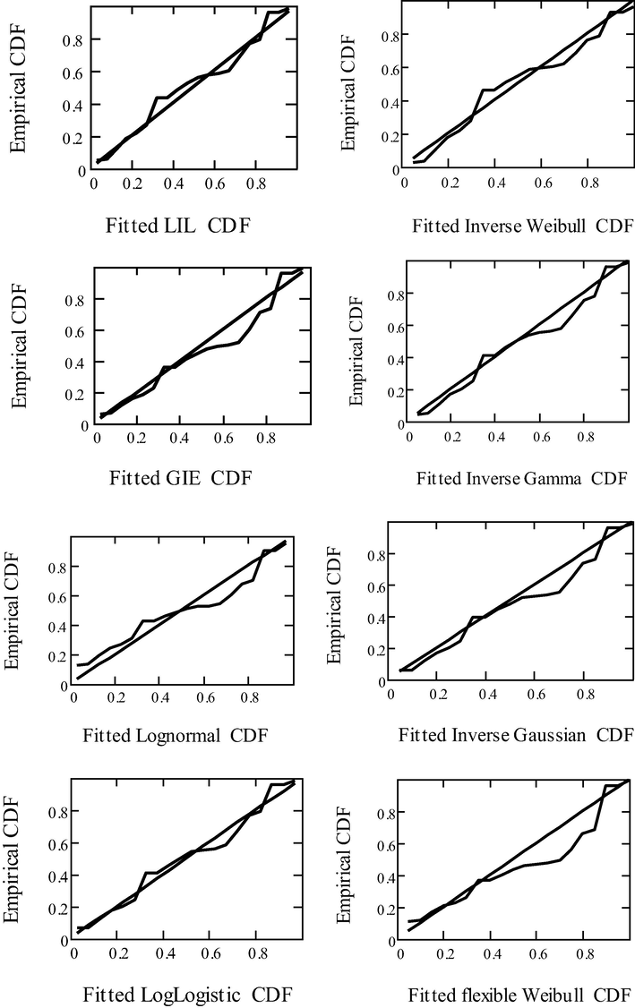
P-P plots for the fitted distributions.

Export to PPT

The goodness-of-fit statistics $W^{\ast }$ and $A^{\ast }$ , are also presented in the tables. These statistics can be used to verify which distribution provides the best fit to the data. In general, the smaller the values of $W^{\ast }$ and $A^{\ast }$ , the better the fit. Let $F(x\text{,}\mathrm{\Theta })$ be the cdf, where the form of $F$ is known but $\mathrm{\Theta }$ (a k-dimensional parameter vector, say) is unknown. To obtain the statistics $W^{\ast }$ and $A^{\ast }$ , we can proceed as follows:

1. Compute $z_i=F(x_i\text{,}\widehat{\mathrm{\Theta }})$ , where the $x_i^{\prime }s$ are in ascending order;

2. Compute $y_i={\mathrm{\Phi }}^{-1}(z_i)$ , where $\mathrm{\Phi }(.)$ is the standard normal cdf and ${\mathrm{\Phi }}^{-1}(.)$ is its inverse;

3. Compute $u_i=\mathrm{\Phi }\{(y_i-\overline{y})/s_y\}$ , where $\overline{y}=(1/n){\sum }_{i=1}^n{y}_i$ and $s_y^2={(n-1)}^{-1}{\sum }_{i=1}^n{(y_i-\overline{y})}^2$ ;

4. Calculate

and $$A^2=-n-\frac{1}{n}{\displaystyle \sum _{i=1}^n}\left\{(2i-1)\ln (u_i)+(2n+1-2i)\ln (1-u_i)\right\}$$ ;Modify $W^2$ into $W^{\ast }=W^2(1+0.5/n)$ and $A^{\ast }=A^2\left(1+\frac{0.75}{n}+\frac{2.25}{n^2}\right)\text{.}$ for more details see (Chen and Balakrishnan (1995)).

We use the likelihood ratio (LR) test statistic to check whether the shape parameter associated with LIL distribution improves its applicability. The hypothesis can be stated as

Null hypothesis $H_0:X\sim \mathit{IL}(\theta )(i.e.\beta =1)$

versus

Alternative hypothesis $H_1:X\sim \text{lIL}(\beta \text{,}\theta )(i.e.\beta \ne 1)$ .

In this case, the LR test statistic for testing $H_0$ versus $H_1$ is ${\omega }^{\ast }=2(l_1-l_0)$ , where $l_1$ and $l_0$ are the log-likelihood functions under $H_1$ and $H_0$ , respectively. The statistic ${\omega }^{\ast }$ is asymptotically

$(\mathit{asn}\to \infty )$ distributed as ${\chi }_k^2$ with $k$ degree of freedom, where $k$ is the number of parameters. The LR test rejects $H_0$ if ${\omega }^{\ast }⩾{\chi }_k^2(\gamma )$ denotes the upper $100\gamma \%$ quantile of the ${\chi }_k^2$ distribution. For given real data set, the log-likelihood under the IL is $l_0=0.5854$ with $\theta =0.6344$ and under H₁, l₁ is 16.4321 with $(\widehat{\beta }=0.0076\text{,}\widehat{\theta }=2.9801)$ . Clearly, the shape parameter $\beta$ can never be 1 for theata since $\widehat{\beta }=0.0076$ which is very far from unity. However, the LR test is ${\omega }^{\ast }=31.6934$ which is greater than ${\chi }_1^2(0.05)=3.84$ . The results indicate that evidences do not support the null hypothesis. Therefore, the LIL is a better model than its special case, IL distribution.

The selection criterion is that the lowest AIC and BIC correspond to the best model fitted. The MLEs, AIC and BIC are shown in Table 3. From the Table 3, we can observed that the LIL distribution shows the smaller AIC and BIC than other competing distributions. Thus, the LIL distribution fits well the data set.

References

- A new customer lifetime duration distribution: the Kumaraswamy Lindley distribution. Int. J. Trade, Economics Finance. 2014;5:441-444.
- [Google Scholar]
- Extended inverse Lindley distribution: properties and application. Springer- Plus. 2015;4:1-13.
- Inferences on stress-strength reliability from Lindley distributions. Commun. Stat. - Theory and Methods. 2013;42:1443-1463.
- A First Course in Order Statistics. Siam, e-books; 1992.
- The inverse Power Lindley distribution. Commun. Statistics - Simulation Computation. 2017;46(8)
- Mathematical Theory of Reliability. Siam, e-books; 1996.
- A general purpose approximate goodness-of-fit. J. Quality Technol.. 1995;27(2):154-161.
- Discrimination between the lognormal and Weibull distribution. Technometrics. 1973;15:923-926.
- Statistical properties of Kumaraswamy quasi Lindley distribution. Int. J. Math. Trends Technol.. 2013;4:237-246.
- Lindley distribution and its application. Math. Comput. Simul.. 2008;78(4):493-506.
- Power Lindley distribution and associated inference. Comput. Stat. Data Anal.. 2013;64:20-33.
- Computer generation of random variables with Lindley or Poisson-Lindley distribution via the Lambert W function. Math. Comput. Simul.. 2010;81(4):851-859.
- Reliability estimation in Lindley distribution with progressively type-ii right censored sample. Math. Comput. Simul. 2011;82:281-294.
- Fiducial distributions and Bayes Theorem. J. Roy. Stat. Soc. Series B (Methodological) 1958:102-107.
- A new method for adding a parameter to a family of distributions with application to the exponential and Weibull families. Biometrika. 1997;84(3):641-652.
- The Lindley distribution applied to competing risks lifetime data. Comput. Methods Programs Biomed.. 2011;104:188-192.
- Transmuted Lindley distribution. Int. J. Open Prob. Computer Sci. Math.. 2013;6:63-72.
- Transmuted Lindley-geometric distribution and its applications. J. Stat. Appl. Probability Lett.. 2014;3:77-91.
- The beta Lindley distribution: properties and applications. J. Appl. Math. 2014:1-10.
- Generalized Poisson-Lindley distribution. Commun. Stat. - Theory Methods. 2010;39:1785-1798.
- A generalized Lindley distribution. Sankhya B - Applied and Interdisc. Stat.. 2011;73:331-359.
- A new class of generalized Lindley distributions with Applications. J. Stat. Comput. Simul.. 2015;85:2072-2100.
- A family of lifetime distributions. Int. J. Quality, Stat Reliability. 2012;2012:1-6.
- A new upside-down bathtub shaped hazard rate model for survival data analysis. Appl. Math. Comput.. 2014;239:242-253.
- The inverse Lindley distribution: a stress-strength reliability model with application to head and neck cancer data. J. Indust. Prod. Eng.. 2015;32(3):162-173.
- The generalized inverse Lindley distribution: a new inverse statistical model for the study of upside-down bathtub data. Commun. Stat.-Theory. Methods. 2016;45(19):5709-5729.
- Load-sharing system model and its application to the real data set. Math. Comput. Simul. 2012;82:1615-1629.
- A two-parameter lifetime distribution with decreasing failure rate. Comput. Stat. Data Anal.. 2008;52:3889-3901.
- The Lindley power series class of distributions: model, properties and applications. J. Comput. Modell.. 2015;5(3):35-80.