

Translate this page into:
Local discontinuous Galerkin method for the nonlocal one-way water wave equation
⁎Corresponding author. mathlican@xaut.edu.cn (Can Li)
-
Received: ,
Accepted: ,
This article was originally published by Elsevier and was migrated to Scientific Scholar after the change of Publisher.
Peer review under responsibility of King Saud University.
Abstract
In this paper, we develop a local discontinuous Galerkin (LDG) method for numerically solving the nonlocal one-way water wave equation. Based on the features of fractional derivative, the considered model is first coupled into a classical first derivative and a nonlocal fractional integral. Then LDG algorithm is used in space discretization by properly choosing the numerical fluxes. Numerical examples are provided to show the accuracy and effectiveness.
Keywords
Nonlocal water wave equation
Local discontinuous Galerkin method

1 Introduction
The study of water waves governed by Euler equations has interested researchers over many years. Under appropriate assumption, the irrotational Euler equations with zero surface tension reduces to the following water wave equation (Wu, 1997; Jennings, 2012; Beale et al., 1993)
Numerical studies of nonlocal water waves equation have been performed in recent works (Chen et al., 2012; Jennings, 2012; Jennings et al., 2014; Li and Zhao, 2016). The LDG method has been intensively studied and successfully applied to solve various linear and nonlinear partial differential equations since it was first introduced by Cockburn and Shu (1998). We refer to Hesthaven and Warburton, 2008, Shu (2016) and references cited therein for the development of LDG methods. Recently, there has been a growing interest in LDG methods for space fractional diffusion problems (Ji and Tang, 2012; Deng and Hesthaven, 2013; Xu and Hesthaven, 2014; Mao and Kamiadakis, 2017). The numerical test results show that the LDG method provides a very effective numerical method for solving nonlocal fractional diffusion equations. Recently, in view of conservative form (1.5), Jennings et al. present a semi-discrete finite volume scheme for (1.5) by using piecewise polynomial reconstruction. Motivated by the work (Ji and Tang, 2012), we will design a highly accurate local discontinuous Galerkin method for the nonlocal conservative form (1.5). The LDG method is constructed by using choosing numerical flux instead of using polynomial reconstruction.
The content of the paper is organized as follows. In Section 2, we present the formulation of the semi-discrete LDG methods for model (1.5). To verify the effectiveness of the proposed LDG scheme, the extensive numerical results are presented in Section 3. Concluding remarks is summarized in Section 4.
2 Formulation of local discontinuous Galerkin method
We design the LDG method for model (1.6) in finite domain
, and we always assume that the solution of model (1.6) has support on
. To design the LDG method for model (1.6), we introduce auxiliary variable
, then the model (1.6) can be rewritten as
Let
be any regular partition of
with mesh step
and
. Denote
and
. The piecewise polynomials of degree at most k over the subintervals
on the cell
is defined as
. The semi-discrete LDG scheme is defined as follows. Find
and
, such that for any
and
,
3 Numerical results
In this section, we present two numerical examples to show the accuracy and the performance of the method for the considered model. In our examples, the condition is used to fulfill the stability. In the first example, we examine the accuracy with piecewise polynomial approximations. The errors are measured by and norms. The computed convergence order are calculated by where is the or -error calculated in the spatial step h. The second example, we simulate the propagation of left and right one-way water wave equations with a special wave packet.
Consider the one-way left-going water wave Eq. (1.6) on the finite domain , . We chose as the exact solution of problem (1.6), and add a source term on the right side of (1.6). The initial-boundary conditions are determined by the exact solution.
Tables 1–2 report the numerical errors and convergence orders for the discrete solutions computed by numerical scheme (2.1). We observe that the accuracy of the LDG scheme are of order
for
, is of order
for
in both
and
norms. In the numerical flux at the boundary, we take
in our computation. To test the stability of the numerical scheme, we rewrite the discrete ODE system (2.2) as
Consider the problem (1.6) with the wave packet (Jennings, 2012; Jennings et al., 2014)
| h | error | order | error | order | error | order |
|---|---|---|---|---|---|---|
| 1/5 | 1.1881e−05 | 2.4200e−06 | 2.0483e−06 | |||
| 1/10 | 3.9638e−06 | 1.5837 | 4.0077e−07 | 2.5942 | 1.0216e−07 | 3.8646 |
| 1/20 | 1.3638e−06 | 1.5393 | 6.4181e−08 | 2.6426 | 5.7122e−09 | 4.3255 |
| 1/40 | 4.6965e−07 | 1.5380 | 1.0403e−08 | 2.6251 | 4.4589e−10 | 3.6793 |
| h | error | order | error | order | error | order |
|---|---|---|---|---|---|---|
| 1/5 | 3.7583e−05 | 7.3163e−06 | 5.0434e−06 | |||
| 1/10 | 1.4405e−05 | 1.3835 | 1.4028e−06 | 2.3828 | 3.7335e−07 | 3.7558 |
| 1/20 | 5.2161e−06 | 1.4655 | 2.3655e−07 | 2.5681 | 1.9811e−08 | 4.2362 |
| 1/40 | 1.7632e−06 | 1.5648 | 3.5806e−08 | 2.7239 | 1.3744e−09 | 3.8494 |
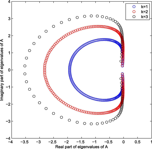
- Eigenvalues of A for
,
, and
.
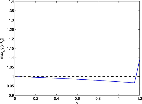
- The distribution of
for
.
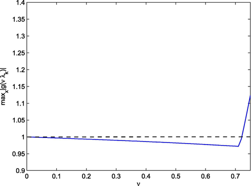
- The distribution of
for
.
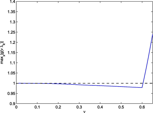
- The distribution of
for
.
The exact solution of (1.6) in not available. To test the effective rate of convergence, we chose
as the “exact” solution which is computed at a fine grid
. The errors and orders of accuracy for numerical solutions are reported in Table 3. We observe that the method with
elements gives a uniform almost
th order of accuracy for LDG solutions in
norm.
h
error
order
error
order
1/40
8.9960e−02
1.1279e−01
1/80
4.1771e−02
1.1068
4.0618e−02
1.4734
1/160
1.4719e−02
1.5048
6.5961e−03
2.6624
We test the wave propagation of the problem (1.6) with wave packet (3.3). The simulation of wave propagation for left and right -going waves are listed in Figs. 5–8. We take
as the computational domain and use the
element with
in our computation. We can see that the moving wave profile is resolved very well. From Figs. 7–8, we can see that the same results can be obtained by using less mesh girds points compared with the method given in Jennings et al. (2014).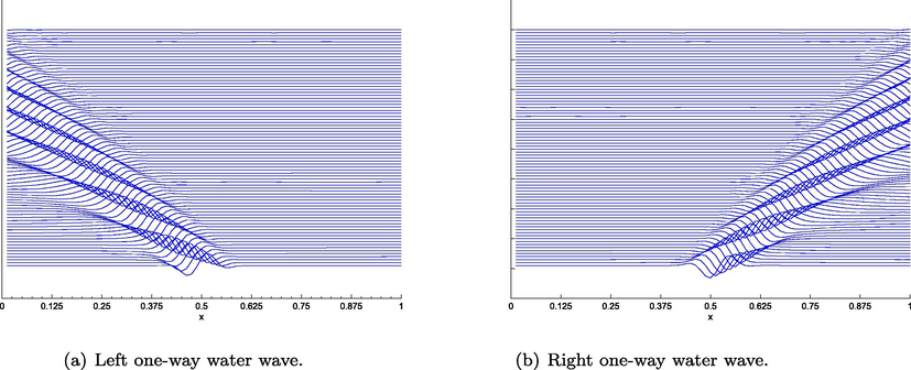
The evolution of left (a) and right (b) going one-way water wave equations with wave packet (3.3).
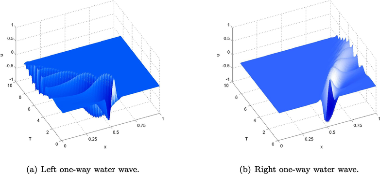
The evolution of left (a) and right (b) going one-way water wave equations with wave packet (3.3).
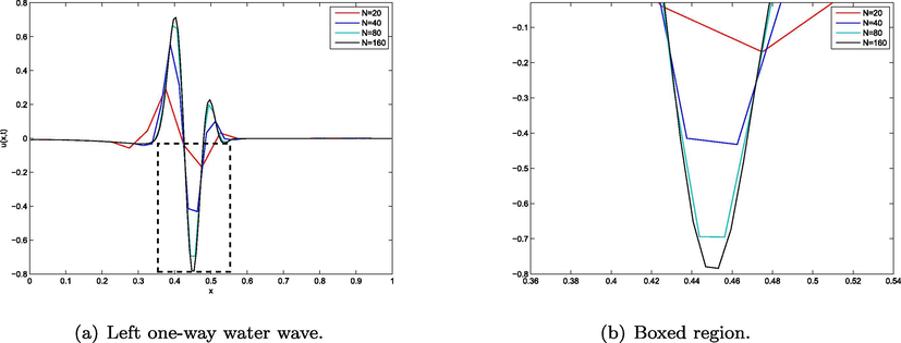
Wave profile for left one-way water waves (a) and boxed region (b) computed by piece wise linear polynomial with wave packet (3.3).
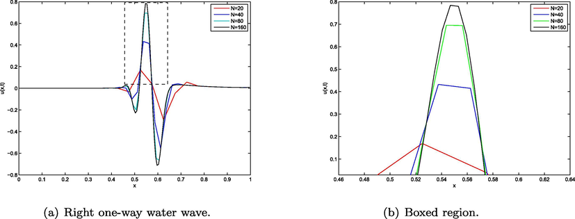
Wave profile for right one-way water waves (a) and boxed region(b) computed by piece wise linear polynomial with wave packet (3.3).
Finally, we discuss the long time behavior of solutions to the one way water wave (1.6) using the LDG method (2.1). It is proved that the solutions of (1.6) decays at the rate
. We compute the solution on the domain
until time
. For
to 100, we compute
. Fig. 9 shows n plotted versus
. From Fig. 9, we can see the numerical solution decays at the rate
, which confirms the theoretical results given by Jennings et al. (2014).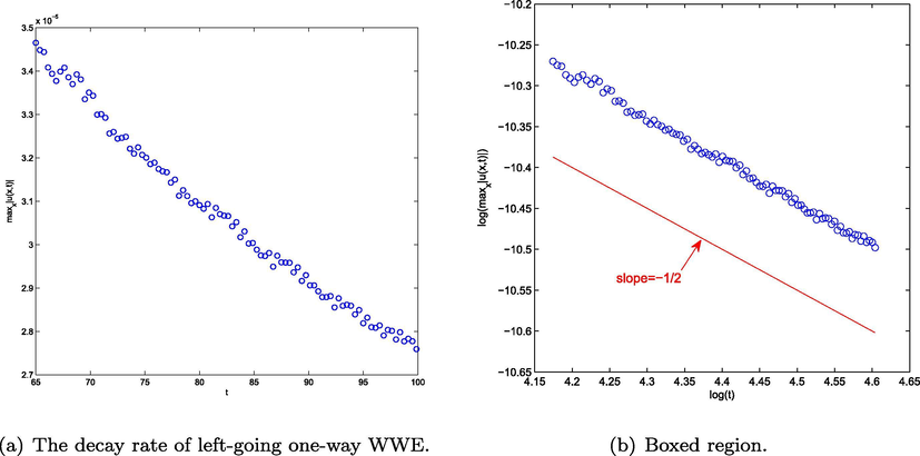
The decay rate of left-going one-way water waves (a) and boxed region (b) computed with initial data (3.3).
4 Conclusion
Inspired by the nature of fractional derivative, we present a local DG methods for the nonlocal one-way water wave equation. The main idea of our method are that the fractional derivative is splitted into a classical first derivative and a nonlocal fractional integral, then the semi-discrete LDG method is designed by carefully choosing the numerical flux. The semi-discrete system is computed by the third order TVD Runge-Kutta method. The numerical scheme is verified for the smooth solution, and some numerical solutions is simulated. Numerical results show that the method with elements don’t give an optimal order of accuracy. We will carry out the details of error estimates in our next work. Finally, numerical simulation shows that our LDG method works well for the one-way water wave equation.
Conflicts of interest
The authors declare that there is no conflict of interests regarding the publication of this paper.
Acknowledgments
We would like to thank the editor and anonymous referees for their many valuable comments and suggestions.
References
- Growth rates for the linearized motion of fluid interfaces away from equilibrium. Commun. Pure Appl. Math. 1993;46(9):1269-1301.
- [Google Scholar]
- Optimal a priori error estimates for the hp-version of the local discontinuous galerkin method for convection-diffusion problems. Math. Comp. 2003;71(238):455-478.
- [Google Scholar]
- Decay of solutions to a viscous asymptotical model for water waves: Kakutani-Matsuuchi model. Nonlinear Anal.: T.M.A. 2012;75(5):2883-2896.
- [Google Scholar]
- The local discontinuous galerkin method for time-dependent convection-diffusion systems. SIAM J. Numer. Anal.. 1998;35(6):2440-2463.
- [Google Scholar]
- Local discontinuous galerkin methods for fractional diffusion equations. ESAIM Math. Model. Numer. Anal.. 2013;47(6):1845-1864.
- [Google Scholar]
- Strong stability-preserving high-order time discretization methods. SIAM Rev.. 2001;43(1):89-112.
- [Google Scholar]
- Nodal Discontinuous Galerkin Methods. Algorithms, Analysis, and Applications. Berlin: Springer; 2008.
- Efficient Numerical Methods for Water Wave Propagation in Unbounded Domains. University of Michigan; 2012. Ph.D. Thesis
- Water wave propagation in unbounded domains. Part II: numerical methods for fractional pdes. J. Comput. Phys.. 2014;275(1):443-458.
- [Google Scholar]
- High-order accurate Runge-Kutta (local) discontinuous galerkin methods for one-and two-dimensional fractional diffusion equations. Numer. Math. Theor. Methods Appl.. 2012;5(3):333-358.
- [Google Scholar]
- Efficient numerical schemes for fractional water wave models. Comput. Math. Appl.. 2016;71(1):238-254.
- [Google Scholar]
- Fractional burgers equation with nonlinear non-locality: spectral vanishing viscosity and local discontinuous galerkin methods. J. Comput. Phys.. 2017;336(1):143-163.
- [Google Scholar]
- Podlubny, I., 1999. Fractional differential equations. an introduction to fractional derivatives, fractional differential equations, some methods of their solution and some of their applications. New York.
- High order weno and dg methods for time-dependent convection-dominated pdes: a brief survey of several recent developments. J. Comput. Phys.. 2016;316(C):598-613.
- [Google Scholar]
- Almost global wellposedness of the 2-d full water wave problem. Invent. Math.. 1997;177(1):45-135.
- [Google Scholar]
- Discontinuous Galerkin method for fractional convection-diffusion equations. SIAM J. Numer. Anal.. 2014;52(1):405-423.
- [Google Scholar]


