Investigation of structural, mechanical, magnetic properties and hysteresis modelling of Dawasir meteorite

1 Introduction

The most cherished geological specimens are commonly known as meteorites due to their presence in the planetary bodies (mostly asteroids). There is no evidence of their accomplishment through manned or unmanned space missions. The main sources of these samples are accidental/incidental meteorite falls. Meteorites are a good scientific resource that provides important information on the diverse collection of terrestrial material, dispersed all over the inner solar system. The earliest meteorite specimens are known as remnants, and were made 4.6 billion years ago in the solar system due to a diverse array of geologic procedures. Meteorites come to the Earth mostly from the outer space, and give information on the solar system itself. This information is relevant to the solar system’s creation, growth and the Earth’s structure. Numerous studies about the celestial history can be obtained from iron-bearing minerals which are essential components of meteorites. These are mainly composed of iron-nickel alloys, and are termed iron meteorites (Oshtrakh et al., 2016). Iron meteorites constitute about 5% of all discovered meteorites. They are denser than the stony meteorites, and constitute about 90% of the total percentage of known meteorites. All of the big meteorites belong to this category. Exomars 2020 has strengthened the expansion of state-of-the-art, non-invasive or semi-invasive investigative diagnostic approaches to study meteorites and similar terrestrial samples on the Earth.

Different researchers around the world have studied the physical, compositional, mechanical, and magnetic properties of different types of meteorites (Bezaeva et al., 2013; Borovička, 2006; Coulson et al., 2007; Duczmal-Czernikiewicz and Michalska, 2018; Flynn, 2005; Flynn et al., 2018; Kohout, 2013; Mercer, 1957; Rubin, 2018; Slyuta, 2017; AlSalhi et al., 2021; Atif et al., 2019; Masilamani et al., 2019). Their studies have covered the meteorites’ mineral composition, the diversity their chemical composition along the contact area, and have provided important clues into the formation and physical evolution of material in the solar protoplanetary disk including indications of the properties of their asteroidal parent bodies. Some studies have provided techniques for the characterization of three-dimensional (spatial) anisotropy, physical and mechanical meteorite properties as well as the distribution of magnetic susceptibility in fragments of the Chelyabinsk ordinary chondrite.

The present sample of high-density meteorite for the investigation belonged to Geophysics Department at the College of Science which was granted by King Faisal Bin Abdulaziz Al-Saud to the Kind Saud University. The picture of the sample is depicted in Fig. 1. It was found and collected by the Saudi Educational Institute’s staff of Wadi Ad Dawasir Province in 1973 during a desert-tour about 25 km north-east of the Al Khamasin desert (20° 36 N, 44° 53 E) (Fig. 2). The importance of Al-Khamasin site of the north western part of Rub’ al-Khali, is an interesting scientific target in KSA due to discovery of the high-density meteorite around 2014. It is pertinent to mention that in Wabar region, a crater was caused by the impact of an iron nickel meteorite and explored by magnetic geophysical survey method. It was concluded that wabar chondrites composed of 92% iron, and about 7.5% nickel, 0.22% cobalt along with iridium element (Gnos et al., 2013; Hofmann et al., 2018). The meteorite sample presented in this study has a very smooth and featureless surface. It often demonstrates shallow depressions clearly visible and a sculptural shape of well-developed regmaglypts that form indentations all over the meteorite’s surface (Fig. 1). The indentations must have formed when the meteorite’s surface was melting during its journey through the atmosphere. The meteorite is a roughly irregular ellipsoid with a cone-shaped mass of brawny and a rusty surface. Its dimensions are 120 cm in length and 75 cm in width. Its total mass is about 2550 kg.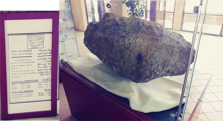

Close

Fig. 1

The Al Khamasin District elucidate meteorite is displayed at the King Saud University.

Export to PPT

Close

Fig. 2

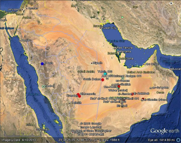
The Al Khamasin Meteorite collection site is located in the desert of Wadi Ad-Dawasir, Saudi Arabia.

Export to PPT

The current study presents the results on the structural modification, mechanical and magnetic properties of the Saudi meteorite. The techniques, applied to examine the meteorite specimen, included field emission scanning electron microscopy (SEM), Energy Dispersive X-Ray Analysis (EDAX), backscattered electron imaging, X-ray powder diffraction (XRD), hardness testing (Rockwell, Vicker, Brinell), and measurements of meteorite magnetic properties.

2 Experimental details

Microscopic studies were carried using SEM JSM-7600F Jeol (Japan). The SEM was equipped with EDX results illustrates morphological and elemental compositional properties. EDX analysis was performed on multiple regions of the specimen in area and point modes using the EDX Oxford system attached to the SEM in order to perform elemental analysis and calculate the elemental contents. The microscopic images were also taken in a backscattered imaging (BSI) mode to observe any regions with varying compositions in the specimen. Later, X-ray diffraction (XRD), using the Bruker D8 Discover Diffractometer, was applied to characterize various phases present in the meteoroid specimen. The XRD was operated at 40 kV and 40 mA with Cu Kα1 radiation (λ = 1.540598 Å), step scan size of 0.02, increment of 1 degree per minute, and a range from 5 to 100°.

Meteorite are kept at 23 °C room temperature conditions protected from dust. To examine the meteorite composition, a small specimen was cut from the bulk of the fallen meteoroid (Fig. 3a). The specimen was then mounted in Bakelite for further testing. Since the specimen was not uniform, it was grinded by a number of silicon carbide disc papers with grit sizes 180, 300 and, finally, 600. It is important to mention that during grinding process some part of the sample remained in its original condition which helped us to compare original surface of the meteorite with the Earth’s atmosphere interaction under microscope analysis.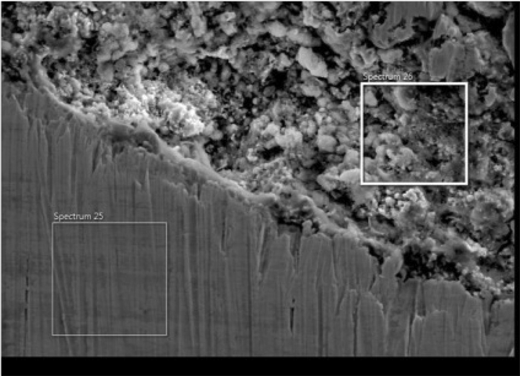

Close

Fig. 3a

The specimens with both modified (grinded) and unmodified (as received) regions are presented.

Export to PPT

To study mechanical properties of the specimen like hardness Zwick/Roel ZHU hardness tester was used. The tester is able to perform various types of hardness tests. The hardness tests performed on the specimen included two Rockwell hardness tests: HRC at 150 kg load and HRA at 60 kg load. A pyramidal diamond indenter was used. In addition, Vicker hardness test (HV) was conducted by using a pyramidal diamond indenter with an angle of 136°. The Brinell hardness test (HB) was performed using a carbide round indenter with a diameter of 2.5 mm.

The EZ7 Vibrating Sample Magnetometer (VSM) was applied to measure the magnetic properties of the specimen. The value of maximum field was 21.5 kOe at 4-mm sized sample. The Magnetometer performed excellently for low coercivity as well as high coercivity measurements due to its high maximum field.

3 Results and discussion

SEM microgram was used to characterize structure of the Saudi meteoroid specimen which is shown in Fig. 3a and Fig. 3d. The specimen was scanned in its initial form (as received) and in its modified form (after grinding with silicon carbide papers with grit sizes 180, 300 and 600). The specimen was grinded to reveal its interior surface that was never in contact with the atmosphere. Fig. 3a depicts SEM microgram of the specimens with modified (grinded) and unmodified regions. The EDAX data of the grinded region demonstrate that iron and nickel are the main constituting elements of the Saudi meteoroid specimen which can be observed from Fig. 3b. The Fig. 3a also reveals that the quantity of iron is very high. However, the EDAX of the unmodified specimen (Fig. 3c) shows that, apart from iron and nickel, various other additional elements, Ca, Mg, Na and O are also detected (Goodrich, 1988). The non-existence of these additional elements in the grinded regions indicates that these elements became part of the specimen as it entered the Earth’s atmosphere, and were added to the specimen after it had entered the Earth’s atmosphere and hit the ground. Upon detailed analysis of the non-grinded regions, it was also found that, unlike any other additional detected elements in the specimen, calcium crystals were present in several places (Fig. 3d) (“Blue crystals in meteorites show that our sun went through the ‘terrible twos,’” 2018; McKeegan et al., 2000). Calcium crystals were randomly distributed and formed agglomerates in some regions. The photograph shows a two-phase region, where one phase is made of calcium crystals and another phase contains iron. It is also noticeable from the SEM microgram depicted in Fig. 3d that some calcium crystals are strongly bonded in-between themselves, however they seem to be poorly bonded with other phase materials. Fig. 3e shows the EDAX of a region containing calcium crystals.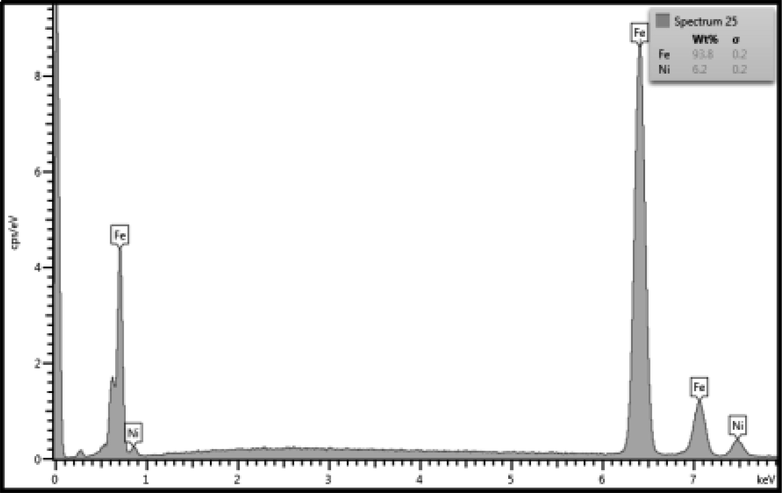

Close

Fig. 3b

The image shows results of the EDAX spectrum of the modified (grinded) region.

Export to PPT

Close

Fig. 3c

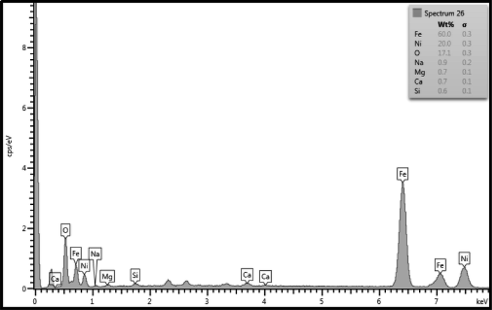
The image shows results of the EDAX spectrum of the unmodified (non-grinded) region.

Export to PPT

Close

Fig. 3d

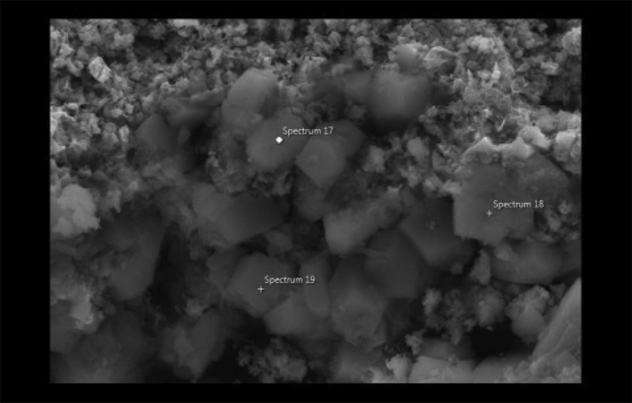
Agglomeration of calcium crystals.

Export to PPT

Close

Fig. 3e

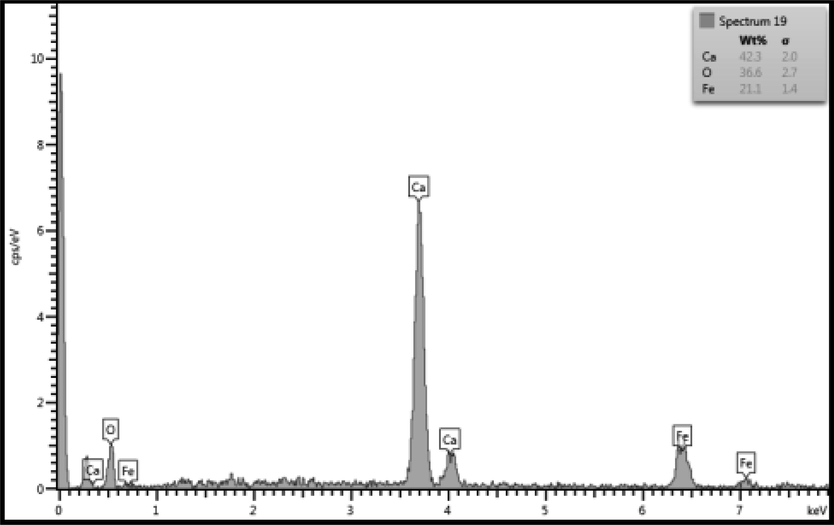
EDAX spot analysis of an agglomerate with calcium crystals.

Export to PPT

The calcium crystals found embedded on the exterior layers of the meteorite are from the impact site. These could be from the calcium carbonate (CaCO3), which is often present in the sand and soil in the form of calcium carbonate mineral phases in surface and subsurface environments in the Earth. Calcium carbonate phases in such environments range from amorphous to crystalline and from anhydrous (calcite, aragonite, and vaterite (CaCO3)) to differently hydrated monohydrocalcite (CaCO3·H2O) and ikaite (CaCO3·6H2O)).

In order to further examine the grinding region, containing iron and nickel, a backscattered electron image was collected (Fig. 4 (a)). The image clearly shows some darker and lighter areas that likely indicate the presence of different phases of iron and nickel. To further investigate the origin of these phases, present in the meteoroid specimen, an XRD analysis was performed using the Bruker D8 Discover Diffractometer. The two theta angles with a range of 5 to 100° with the scan speed of 1 degree per minute, and a 0.02 degree per minute increment were used. The source was the copper K-Alpha 1.540 with the voltage of 40 KV and 40 mA. The major phase, identified from the XRD analysis, was the mineral kamacite (Fig. 4(b)). Kamacite is an alloy of iron and nickel, and has been previously identified in the meteoroid specimens collected from different places of the Earth (Goldstein and Goddard, 1965).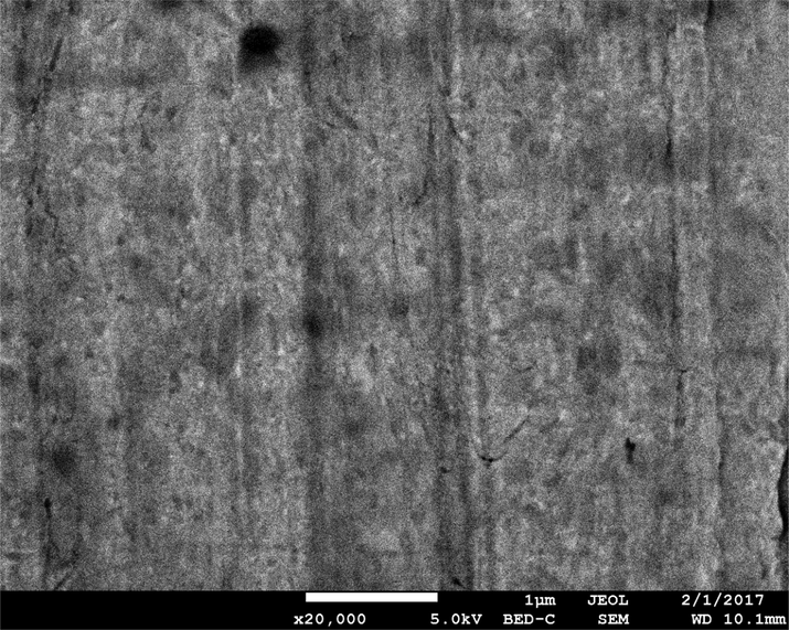

Close

Fig. 4a

Backscattered electron image of the meteorite specimen.

Export to PPT

Close

Fig. 4b

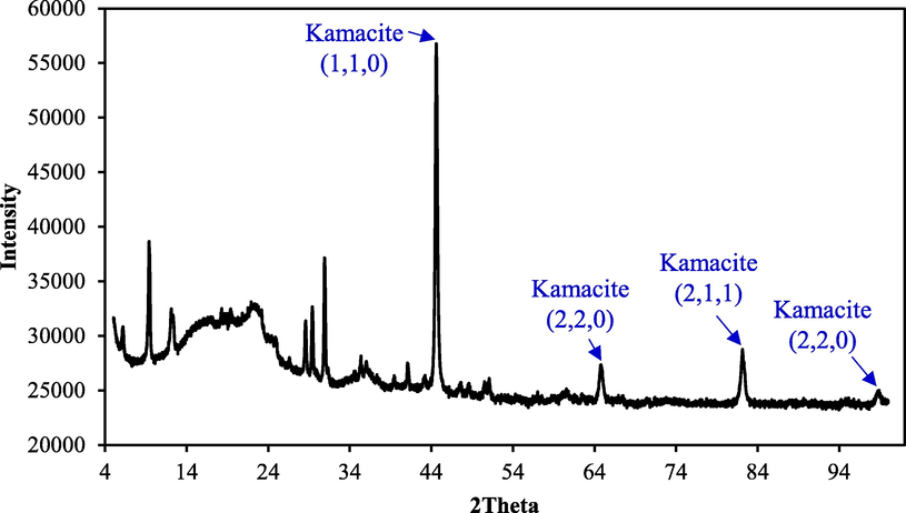
XRD spectra of the meteoroid specimen.

Export to PPT

Fig. 5 shows the results of the hardness test measurements carried out on the specimen, whereas Table 1 summarizes different results of the hardness test values. From the hardness tests, it appears that the meteoroid is composed of a relatively soft material (Table 1). Moreover, this material does not belong to the high-regime of hardness values after comparison with different categories of iron alloys (steels).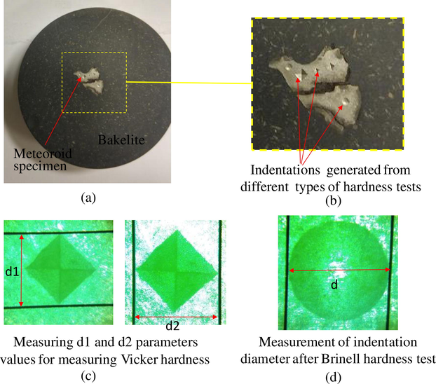

Close

Fig. 5

(a) Meteoroid specimen mounted in Bakelite. (b) Zoomed-in view of the specimen after completion of several hardness tests. (c) Micrographs of indentations generated after the Vicker hardness test. (d) Micrograph of indentations generated after the Brinell hardness test.

Export to PPT

The HRB hardness values (Table 1) closely match the stainless-steel grades 301 (HRB 95) and 310 (HRB 95), containing 6–8% of Ni and 19–22% of Ni, respectively. These steel grades are usually regarded as less hard steel grades (see the websites at the end of the reference section). It should be noted that in these references the HRB hardness scale is used for hardness testing, and is commonly employed for softer materials.

The magnetic properties of the studied material were examined at room temperature using the Physical Property Measurement System (PPMS) under the influence of an applied magnetic field of 6 kOe (Fig. 6). The sample shows a soft-material behavior as do the ferromagnetic materials. It was also noticed that the material is not fully saturated in the given magnetic field. The magnetic saturation (M_s) of 0.701 emu/g was observed for the saturation field of (H_s) = 5025 Oe. The resonant magnetization (M_R) of 0.146 emu/g was observed with a low coercive field (H_c) of 150.94 kOe. These observations are in good agreement with the previously reported data from ordinary chondrites (Gattacceca et al., 2011). In summary, this study on the structural modification, mechanical and magnetic properties of the Saudi meteorite confirm the iron-nickel meteorite composition.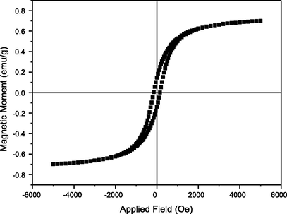

Close

Fig. 6

Hysteresis loops: the applied field dependencies of magnetization recorded at room temperature.

Export to PPT

4 Mathematical modeling

The data is obtained from the experimental studies of physical properties measurement system (PPMS) under the influence of magnetic field of 6KOe. This data is partitioned into four equal portions. These portions are highlighted in the Fig. 7(a). 2nd Portion is selected for the mathematical modelling and the comparison purpose. 4th portion of the data is replica of 2nd portion and can be modelled with symmetrical process. Similarly, 1st portion is odd symmetric to the 3rd portion of the data. It happens in every hysteresis loop and the advantage of symmetry can be claimed in all types of such curves.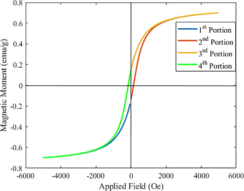

Close

Fig. 7a

Experimental data measured by variation of applied field (Oe) and observing the Magnetic moment (emu/g) for the sample of meteoroid under test. Data is further divided in 4 segments where, 2nd segment is selected for mathematical modelling.

Export to PPT

In order to model such hysteresis loop, many efforts are being performed in literature (Barton, 1933; El-Sherbiny, 1973; Emery, 1892; Faiz, 2001; Rivas et al., 1981; Trutt et al., 1968; MacFadyen et al., 1973; Brauer, 1986; Geyger, 1965) proposes the hysteresis loop modelling techniques and hysteresis loss estimation of soft magnetic materials. Sinusoidal function was used to evaluate the goodness of fit and inverse sine function was proposed for the representation of hysteresis loss. (Włodarski et al., 2005) tied three different models like cot hyperbolic function, tan^-1 model and frohlich (froelich) model for fitting the data of hysteresis. (Dadic et al., 2020) presented a comprehensive analysis of already existing models present in the literature and proposed complex exponential model with 100 order is best for modelling. However, it requires lot of constants to model the hysteresis data. In this model a comprehensive analysis is proposed with lesser number of coefficients with acceptable error.

The most common function available to model the hysteresis data is Frohlich function a generalized form of Frohlich function is shown in equation (1).

The second most common function in the literature is the inverse tan function that can model hysteresis is shown in equation (2).

There are few other forms of common functions that can fit such data. One of the other common function is erf(x) function as shown in equation (3)

Table 2 shows all the unknown constant extracted from the method of least square errors along with the values of parameters of goodness of fit. The models described from equation (1) to equation (8) are implemented on Matlab using Levenberg-Marquardt algorithm for non-linear regression process.

Fig. 7(b) shows the estimation of 2nd portion of hysteresis data with optimized values of unknown constants listed in Table 2. The optimized values of unknown constants are extracted using Levenberg-Marquardt algorithm for non-linear regression process. Different functions are used for the estimation of hysteresis data in this Fig. 6 such as Frohlich function, tan-1 function, Modified erf function and modified logistic functions. It is observed that the modified logistic function or log sigmoid function is closest to the experimental data.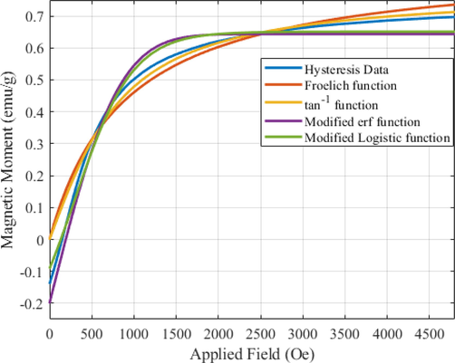

Close

Fig. 7b

2nd portion of the Hysteresis data is compared with the existing models such as Frohlich function, tan-1 function, Modified erf function and modified logistic functions.

Export to PPT

Fig. 7(c) shows the modelling of hysteresis data with modified frohlich function, simple exponential function and bi-exponential function. It can be observed that the bi-exponential model is almost overlapping the experimental data. Other candidate functions are close to the experimental data with some error. The difference between the experimental data and the candidate function is measured point by point subtraction. While the other errors can be described with single figure of merit like RMSE, SSE, R-square and Adjusted R-square.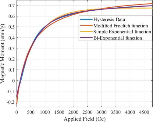

Close

Fig. 7c

2nd portion of the Hysteresis data is compared with the existing models such as Modified Frohlich function, simple exponential function and Bi-Exponential function.

Export to PPT

Root Means Square Error (RMSE) criteria is defined as in equation (9).

Sum of Square of Error (SSE) criteria is defined in equation (10).

R-square is another measure of goodness of fit as shown in equation (12)

Adjusted R-square is also calculated for each of the candidate function via equation (12).

It can be observed that the relation between Applied field (H) and magnetic moment (B) can be expressed in equation (13)

All these errors are also calculated to show the goodness of fit and listed in Table 2.

Fig. 8(a) shows the point to point difference between the candidate function and the actual hysteresis data. It can be seen that modified logistic function is close to zero while other functions are away from zero axis. This shows that the modified logistic function outperforms modified erf function, tan^-1 and Froelich function.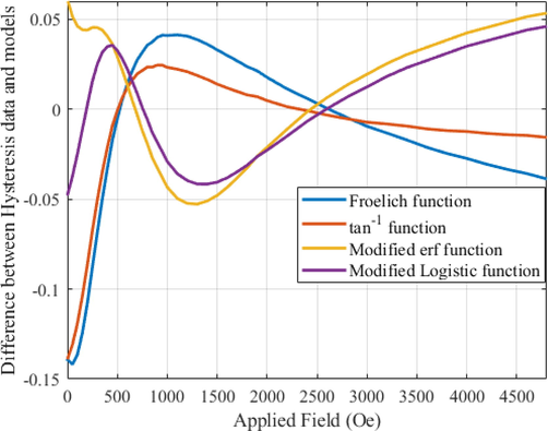

Close

Fig. 8a

Difference between Hysteresis data with different proposed models such as Frohlich function, tan-1 function, Modified erf function and modified logistic functions, for highlighting better goodness of fit.

Export to PPT

Fig. 8(b) shows the point to point difference between the candidate function and hysteresis data. It can be observed that bi-exponential model is close to zero while other functions are away from zero. this figure shows that bi-exponential model outperforms all the other functions. Other errors shown from equation (9) to equation (12) are also calculated and listed in Table 2.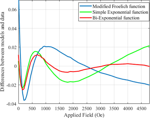

Close

Fig. 8b

Difference between Hysteresis data with different proposed models such as Modified Frohlich function, simple exponential function and Bi-Exponential function, for highlighting better goodness of fit.

Export to PPT

It can be noticed that (Dadic et al., 2020) requires 200 coefficients to model hysteresis in order to produce lower order of RMSE while this work proposed only four coefficients to produce reasonably low RMSE. Hence, the model produced with equation (8) are in good agreement with the hysteresis data.

5 Conclusion

Investigation of the structural modification, mechanical and magnetic properties of the massive meteorite from Saudi Arabia is presented. The conducted analyses show that the meteorite is a celestial iron-nickel alloy formed under unknown temperature and pressure conditions. The meteorite likely experienced rapid heating and cooling as it trans versed the outer space. A number of modern techniques, such as XRD and SEM, were applied in order to investigate the metallurgical and other properties of the strange alloy. This showed that the sample is essentially an iron-Ni alloy. The SEM surface morphology analysis revealed the distribution/agglomeration of the contaminants and the parent elemental/phase distribution. In addition, the surface hardness tests (Vicker, Rockwell, Brinell) were carried out and revealed that this alloy is relatively soft and has little, if any, martensite formation. The hardness test confirmed that the meteorite is composed of a soft material with 22.5 HRC Rockwell hardness. The measurement of a meteorite ferromagnetic field of 6 kOe indicates a soft-material behavior as ferromagnetic materials tend to display. The value of magnetic saturation (M_s) of 0.701 emu/g with a saturation field of (H_s) = 5025 Oe was calculated using a BH curve. The value of resonant magnetization (M_R) of 0.146 emu/g was perceived at a low coercive field (H_c) of 150.94 kOe. Mathematical modeling of the hysteresis data is performed using different function available in the literature, few modified functions are also proposed and evaluated for the goodness of fit. Different figure of merits is calculated to show the best function for the fitting of hysteresis data. It is concluded that bi-exponential function outperforms all the existing models with fewer number of coefficients. Increasing the number of exponentials more than 2 will not decrease the errors significantly. Hence bi-exponential model is a reasonable choice for modeling hysteresis data along with lesser number of coefficients.

References

- Elemental composition and physical characteristics of the massive meteorite of the Saudi empty quarter. J. King Saud Univ. - Sci.. 2021;33
- [Google Scholar]
- Atif, M., Anwar, S., Farooq, W.A., Ali, M., Masilaimani, V., AlSalhi, M.S., Abuamarah, B.A., 2019. Study of the Compositional, Mechanical and Magnetic Properties of Saudi Meteorite. https://doi.org/10.1007/978-3-030-01575-6_19.
- Empirical equations for the magnetization curve. Trans. Am. Inst. Electr. Eng.. 1933;52:659-664.
- [CrossRef] [Google Scholar]
- Magnetic properties of the Chelyabinsk meteorite: Preliminary results. Geochemistry Int. 2013;51:568-574.
- Blue crystals in meteorites show that our sun went through the “terrible twos,” 2018. . F. Museum.
- Properties of meteoroids from different classes of parent bodies. In: Proceedings of the International Astronomical Union. 2006.
- Brauer, J., 1986. Simple equations for the magnetization and reluctivity curves of steel 107, 272.
- Physical properties of Martian meteorites: porosity and density measurements. Meteorit. Planet. Sci.. 2007;42
- Approximation of the nonlinear B-H curve by complex exponential series. IEEE Access. 2020;8:49610-49616.
- Mineralogy and microstructure of the Morasko meteorite crust. Planet. Space Sci. 2018
- Representation of the magnetization characteristic by a sum of exponentials. IEEE Trans. Magn.. 1973;9:60-61.
- Rational and empirical formula showing the relation between the magneto-force (H) and the resulting matnetization (H) Trans. Amer. Inst. Elect. Eng.. 1892;9:192-222.
- Hysteresis loop modeling techniques and hysteresis loss estimation of soft magnetic materials. COMPEL – Int. J. Comput. Math. Electr. Electron. Eng.. 2001;20:988-1002.
- Physical properties of meteorites and interplanetary dust particles: clues to the properties of the meteors and their parent bodies. Earth Moon Planets 2005
- Physical properties of the stone meteorites: implications for the properties of their parent bodies. Chemie der Erde. 2018;78
- Low temperature magnetic transition of chromite in ordinary chondrites. Geophys. Res. Lett. 2011
- Geyger, W.A., 1965. Nonlinear-Magnetic Control Devices: Basic Principles, Characteristics and Applications.
- The Wabar impact craters, Saudi Arabia, revisited. Meteorit. Planet. Sci. 2013
- The formation of the Kamacite Phase in metallic meteorites. J. Geophys. Res.. 1965;70:6223-6232.
- Meteorite reconnaissance in Saudi Arabia. Meteorit. Planet. Sci.. 2018;53
- Physical properties of the Chelyabinsk meteorite. In: 76th Annu Meteorit. Soc. Meet.. 2013.
- Masilamani, V., Alarif, N., Farooq, W.A., Atif, M., Ramay, S., Althobaiti, H.S., Anwar, S., Elkhedr, I., AlSalhi, M.S., Abuamarah, B.A., 2019. Physical characteristics of the massive meteorite of Saudi empty quarter. https://doi.org/10.1007/978-3-030-01575-6_18.
- Incorporation of short-lived 10Be in a calcium-aluminum-rich inclusion from the Allende meteorite. Science (80-) 2000
- Iron sulfide (troilite) inclusion extracted from Sikhote-Alin iron meteorite: Composition, structure and magnetic properties. Mater. Chem. Phys. 2016
- Simple approximation for magnetization curves and hysteresis loops. IEEE Trans. Magn.. 1981;17:1498-1502.
- Carbonaceous and noncarbonaceous iron meteorites: differences in chemical, physical, and collective properties. Meteorit. Planet. Sci. 2018
- Physical and mechanical properties of stony meteorites. Sol. Syst. Res.. 2017;51:64-85.
- Representation of the magnetization characteristic of DC machines for computer use. In: IEEE Trans. Power Appar. Syst. PAS-87. 1968. p. :665-669.
- W. K. MacFadyen, R. R. S. Simpson, R. D. Slater, W.S.W., 1973. Representation of magnetisation curves by exponential series. Proc. Inst. Elect. Eng 120, 902–904.
- Application of different saturation curves in a mathematical model of hysteresis. COMPEL – Int. J. Comput. Math. Electr. Electron. Eng.. 2005;24:1367-1380.
Appendix A
Supplementary data
Supplementary data to this article can be found online at https://doi.org/10.1016/j.jksus.2022.101902.
The following are the Supplementary data to this article: