

Translate this page into:
Interval linear algebra – A new perspective
⁎Corresponding author. ganesank@srmist.edu.in (K. Ganesan)
-
Received: ,
Accepted: ,
This article was originally published by Elsevier and was migrated to Scientific Scholar after the change of Publisher.
Peer review under responsibility of King Saud University.
Abstract
The purpose of this article is to put the concept of interval linear algebra on a sound algebraic setting, by judiciously defining a Field and a Vector Space over a field involving equivalence classes. Classifying mathematical objects by bringing them into canonical forms, is an important subject of study in every branch of Mathematics. The concepts of eigenvalues and eigenvectors are used in several fields including machine learning, quantum computing, communication system design, construction design, electrical and mechanical engineering etc. The study of interval matrices leads to canonical forms of interval matrices, which will help us classify and study interval matrices more effectively and more easily.
Keywords
Interval
Interval matrix
Equivalance relation
Eigenvalues
Eigenvectors
Canonical forms

1 Introduction
A real life problem can be formulated as a mathematical model involving matrices, system of linear and nonlinear equations, ordinary and partial differential equations and linear and nonlinear programming problems etc. When the decision parameters of the model are well-known precisely, the classical mathematical techniques and methods are used successfully for solving such problems. But, in real world situations, the decision parameters are unlikely to be certain due to many reasons like errors in data, inadequate information, errors in formulation of mathematical models, changes in the parameters of the system, computational errors etc. Hence, in order to model the real-world problems and perform computations, the uncertainty and inexactness must be dealt with. We cannot successfully use traditional classical mathematical techniques for modeling real world problems. However, probability theory, theory of fuzzy sets, theory of interval mathematics and theory of rough sets etc deal with the uncertainty and inexactness successfully. The uncertainties in a problem have to be represented suitably so that their effects on present decision making can be properly taken into account. In fuzzy approach, the membership function of fuzzy parameters and in stochastic approach, the probability distribution of decision parameters have to be made known. But, in real life situations, it is not simple to define the membership function or probability distribution in an inexact environment. Therefore, the use of intervals is more appropriate to an inexact environment. Intervals are efficient and reliable tools allowing us to handle such problems effectively.
The role of matrices is all encompassing and ubiquitous in all disciplines. Hansen and Smith (1967) initiated the importance of interval arithmetic in matrix computations. Motivated by this, many authors Alefeld and Herzberger (1983), Deif (1991a), Ganesan and Veeramani (2005), Ganesan (2007), Goze (2010), Sengupta and Pal (2000), Jaulin et al. (2003), Neumaier (1990), Singh and Gupta (2015) etc have studied interval matrices. Hansen (1969, 1992), Hansen and Walster (2004) discussed the solution of linear algebraic equations with interval coefficients and the global optimization using interval analysis.
Deif (1991a) introduced the characterization of the set of eigenvalues of a general interval matrix and obtained the upper and lower bounds of the eigenvalues. Ganesan and Veeramani (2005) proposed a new type of arithmetic operations on interval numbers. Ganesan (2007) studied some important properties of interval matrices. Sunaga (2009) investigated the algebraic properties of intervals, interval functions and functionals and their derivatives. Singh and Gupta (2015) applied the interval extension of the single step eigen perturbation method and obtained sharp eigenvalue bounds for real symmetric interval matrices by solving the standard interval eigenvalue problem. The deviation amplitude of the interval matrix is considered as a perturbation around the nominal value of the interval matrix. Nerantzis and Adjiman (2017) have presented a branch-and-bound algorithm for calculating bounds on all individual eigenvalues of a symmetric interval matrix. Qiu and Wang (2005) evaluates the upper and lower bounds on the eigenvalues of the standard eigenvalue problem of structures subject to severely deficient information about the structural parameters. Gavalec et al. (2020) have studied three types of interval eigenvectors namely the strong, the strongly universal, and the weak interval eigenvector of an interval matrix in max-plus algebra. Sit (2021) studied some properties of interval matrices. The author also established some theoretical results on the regularity and the singularity of an interval matrix using eigenvalues of the interval matrix. Qiu et al. (1996, 2001, 2005) have studied eigenvalue problems involving uncertain but non-random interval stiffness and mass matrices. They proposed an approximate method for estimating the bounds of eigenvalues of the standard interval eigenvalue problem of the real non-symmetric interval matrices and also the eigenvalue bounds of structures with uncertain-but-bounded parameters. Also, several authors (Deif, 1991b, Hertz, 1992, Kolev, 2006, Leng and He, 2007, Rump and Zemke, 2004, Wilkinson, 1961, Yamamoto, 2001, Yuan et al., 2008) contributed to the study of interval eigenvalue problems.
In this article, we introduce new pairing techniques and arithmetic operations on intervals in and interval matrices in . This paper sets the tone for canonicalization of interval matrices by determining the most important characteristics of an interval matrix namely, interval eigenvalues and interval eigenvectors. The specialty of the approach mentioned in this paper is that the interval eigenvalues and normalized interval eigenvectors are uniquely determined. We discuss an electric circuit problem under uncertainty described by a system of interval linear differential equations. Numerical examples are provided to illustrate theory developed in this paper.
This paper is arranged as follows: Section 1 is the introduction part. Section 2 provides some basic necessary preliminaries and results about closed intervals on the real line. Section 3 contains the main work on interval linear algebra and in Section 4, some examples are discussed using the proposed method. Section 5 deals with a real world application of the proposed method on electric circuit theory under uncertain environment which is modeled as a system of interval linear differential equations. Finally, a brief conclusion is given in Section 6.
2 Preliminaries
Let be the set of all closed and bounded intervals. If , then is a degenerate interval.
The intervals are identified with an ordered pair defined as follows: Let . Define and and hence can be uniquely expressed as . Conversly, when is known, then and of and hence given , the interval is unique.
Note: If , then is said to be a zero interval. In particular, if and , then . If and , then . It is to be noted that if , then , but the converse need not be true. If , then is said to be a non-zero interval. If then is said to be a positive interval and is denoted by .
2.1 Arithmetic operations on intervals
We define a new type of arithmetic operations on intervals through their mid points and widths. Mid points follows the usual arithmetic on and the widths are following the lattice rule which is least upper bound and greatest lower bound in the lattice L. That is for and .
For any two intervals , and , the arithmetic operations are defined as In particular for and in , We have
-
Addition:
-
Subtraction:
-
Multiplication:
-
Division: , provided .
Ganesan and Veeramani (2005) For any two and in , we have
and .
and .
and if or .
and , where .
2.2 Exponentiation of intervals
In certain applications, the exponentiation of intervals play a key role in arriving at the solution. So we can define the exponential of intervals as follows.
For any interval , we define .
Result. For any two intervals , we have and . Therefore That is .
3 Interval linear algebra
For all , define if . Then this relation is an equivalence relation on .
Proof: For any . Hence . Thus R is Reflexive.
Let and . Hence , Thus R is Symmetric.
Let with and . Then and . Hence which implies . Thus R is transitive. Hence R is an Equivalence Relation.
Note: Let be the set of all equivalence classes of intervals under the equivalence relation R on and all intervals in an equivalence class will have the same mid point say . We denote this equivalence class by and will be identified with m (or) with where is any closed interval in .
On E, we define a binary operation +, called addition as follows:
Take . Define . We note that + is well defined on E and is indeed a binary operation on E.
Define another binary operation on E called multiplication as follows:
For all , we define . We note that on LHS is a definition on E and on RHS, denotes the usual multiplication of real numbers. is well defined on E and turns out to be a binary operation on E. We may write interchangeably as as in the case of multiplication of real numbers.
Any real number can be converted into an interval by choosing any non-negative real number and defining . This non-negative real number is said to pair with .
In this paper, the crisp eigenvalues and crisp eigenvectors of are converted into interval eigenvalues and interval eigenvectors of by judiciously choosing the pairing number in such a way that the interval eigenvalues and normalized interval eigenvectors are unique.
is a field.
Proof: Let .
(i). (by definition). Sum of two real numbers is which is also a real number and hence . Hence ’addition’ in E has closure property.
(ii). Since addition in is associative, we have .
(iii). and hence and . Hence is the identity on E and we will call this identity as the additive identity on E.
(iv). Let , then and so which gives . Also . Similarly . Thus we conclude that is the additive inverse of .
(v). Let and hence we have the commutativity of + on E.
(vi). Product of two real numbers is a real number and hence for all . Hence has closure property on E.
(vii). Product (usual multiplication) of real numbers is associative and hence . Hence is associative in E.
(viii). . Therefore and . Therefore is the identity (multiplicative identity which we will also call as unity) in E.
(ix). Let . Then . So and . Hence all non-zero elements in E have a multiplicative inverse in E.
(x). . Therefore multiplication is commutative in E.
(xi). . Hence multiplication in E distributes over addition in E.
Thus E is a Field for the two binary operations + and .
(Frobenius-Perron) Strang (2003) Let A be an matrix with non-negative entries. Then the following are true:
-
A has a non-negative real eigenvalue. The largest such eigenvalue, , dominates the absolute values of all other eigenvalues of A. The domination is strict if the entries of A are strictly positive.
-
If A has strictly positive entries, then is a simple positive eigenvalue, and the corresponding eigenvector can be normalized to have strictly positive entries.
-
If A has an eigenvector with strictly positive entries, then the corresponding eigenvalue is .
E and are isomorphic as fields by the natural isomorphism which associates to .
Proof: Define by , for all . This f is well defined on E since the midpoint of any interval in an equivalence class is the same. Also . Therefore f is additive on E (i.e. f preserves addition on E). Now . Hence f is multiplicative on E. That is f preserves multiplication on E.
Claim (i): f is (injective).
. Hence f is injective.
Claim (ii): f is onto (surjective).
and and hence f is surjective. Thus f is a bijective Ring homomorphism between the fields E and which leads us to conclude that E is isomorphic to . That is .
Note: This isomorphism enables us to identify an element of E (an equivalence class) with a real number which is the mid point of any interval in the equivalence class.
Using the identification between intervals and ordered pairs (i.e. and ), we get unique solutions to interval equations, eigenvalues and eigenvectors of interval matrices which in turn leads to canonical forms of interval matrices.
The field isomorphism between E and enables us to convert interval matrices into classical matrices. After finding the eigenvalues and normalized eigenvectors for these classical matrices formed by mid points and widths of intervals, we get interval eigenvalues and normalized interval eigenvectors for the given interval matrices. This is illustrated by examples (1) and (2).
3.1 Interval matrices
A classical matrix is a rectangular array of elements of a field . whenever impreciseness or uncertainty occurs in the entries of a matrix, we switch over to Interval matrices, where each entry of the matrix is a closed and bounded interval in .
An interval matrix is a matrix whose entries are closed and bounded intervals and is denoted by = = , where each .
We use to denote the set of all equivalence classes of interval matrices. By we denote a matrix whose entries are the corresponding midpoints of the entries of . i.e. = . The width of an interval matrix is the matrix of widths of its interval elements defined as = , where each entry of is always non-negative. We use O to denote the null matrix and to denote the null interval matrix . Also we use I to denote the identity matrix and to denote the identity interval matrix .
In particular if and , then.
= .
An interval vector is a column vector whose components are closed intervals. We use to denote the set of all n-dimensional interval vectors. By we denote a vector whose entries are the corresponding mid points of the entries of . i.e) and the width of interval vector is defined by .
3.2 Interval matrix operations
If , where and , then
3.3 Eigenvalues and eigenvectors of interval matrices
Let be an interval matrix. A non-zero interval vector satisfies for some is said to be an interval eigenvector of and such is called an interval eigenvalue of .
Note: In the case of interval matrices , we note that the width matrix contains only non-negative entries. Hence the Perron-Frobenius Theorem for such matrices guarantees the existence of a non-negative eigenvalue for the width matrix which in turn will give a unique eigenvalue for an interval matrix corresponding to every real eigenvalue of . The hallmark of this procedure is that the set of eigenvalues obtained for a given interval matrix is unique.
is an interval matrix.
(a). Corresponding to every real eigenvalue of , we get a unique interval eigenvalue for .
(b). Corresponding to every normalized eigenvector for eigenvalue , we get a unique normalized interval eigenvector for .
Proof: (a). Let be a real eigenvalue of . Find all eigenvalues of . Two cases arise.
Case (i): has a positive eigenvalue. In this case, we take The pair will give a unique interval eigenvalue of namely .
Case (ii): If does not have positive eigenvalue, the non-negativity of the entries of ensures the applicability of the Perron-Frobenius theorem for and hence the matrix is nilpotent. Hence all eigenvalues of are zero which implies that the interval eigenvalues of is degenerate.
(b). The unique interval eigenvector corresponding to is computed as follows:
Let be the normalized eigenvector of corresponding to the eigenvalue . Find the normalized eigenvector corresponding to given in case(i) or corresponding to 0 which arises in case(ii). Since an eigenvector is non-zero and and are normalized eigenvectors for the same eigenvalue . For a normalized eigenvector of , define Pairing this with will produce the unique interval eigenvector .
In case the geometric multiplicity of an eigenvalue , then the k crisp normalized eigenvectors corresponding to form an rectangular matrix say . In this case The k normalized eigenvectors corresponding to give a unique set of k linealy independent interval eigenvectors. Again we can ensure the interval eigenvectors to be unique with the same geometric multiplicity. Hence the theorem.
3.4 Algorithm for eigenvalues and eigenvectors of an interval matrix
Given an interval matrix .
Step (1). Find and .
Step (2). Find eigenvalues of and over .
Step (3). Find is an eigenvalue of . By Perron-Frobenius, there exist a minimum positive eigenvalue for is failing which is nilpotent.
Step (4). Corresponding to every real eigenvalue of ,we consider the pair ( ) to find interval eigenvalues for . In case is nilpotent the crisp real eigenvalues of give degenerate interval eigenvalues for .
Step (5). Find the normalized eigenvectors corresponding to every real eigenvalue of and the normalized eigenvector corresponding to of . In this case, the eigenvector pairing number is , where of .
Step (6). When the geometric multiplicity of an eigenvalue ,then the k crisp normalized eigenvectors corresponding to form an rectangular matrix say . In this case, the eigenvector pairing number is .
The k normalized eigenvectors corresponding to give a unique set of k linealy independent normalized interval eigenvectors, thus exhibiting the same geometric multiplicity for the crisp and interval eigenvalues.
4 Numerical examples
Find the eigenvalues and eigenvectors of the interval matrix
Solution: Consider the midpoint matrix . The eigenvalues of are and the corresponding normalized eigenvectors are . Also consider the width matrix . The eigenvalues of are . Both eigenvalues are positive, so choose minimum positive eigenvalue 0.14 and the corresponding normalized eigenvector is . Here is an eigenvector and hence is also an eigenvector and in order to reach absolute minimum, we consider as the normalized eigenvector.
Now the unique interval eigenvalues of the given interval matrix are:
This is justified because we are interested in minimising vagueness or error. The interval eigenvalues of the given interval matrix are and . The normalized interval eigenvectors of the given interval matrix are computed as follows:
Case 1: The normalized interval eigenvector corresponding to the interval eigenvalue is since is the absolute minimum. Hence for the interval eigenvalue , the corresponding normalized interval eigenvector is .
Case 2: The normalized interval eigenvector corresponding to the interval eigenvalue is Hence for the interval eigenvalue , the corresponding normalized interval eigenvector is . From the above cases, we see that, the interval eigenvalues of are and and the corresponding normalized interval eigenvectors are and .
Find the eigenvalues and eigenvectors of the symmetric interval matrix
Solution: Consider midpoint matrix . The eigenvalues of are and the corresponding normalized eigenvectors are . Also consider width matrix . The eigenvalues of are . Here choose positive eigenvalue 2.50 and the corresponding normalized eigenvector is .
Now the unique interval eigenvalues of the given interval matrix are:
Therefore the interval eigenvalues of are and .
The normalized interval eigenvectors of the given interval matrix are computed as follows:
Case 1: The normalized interval eigenvector corresponding to the interval eigenvalue is , since is the absolute minimum. For the eigenvalue , the corresponding normalized eigenvector is .
Case 2: The normalized interval eigenvector corresponding to the interval eigenvalue of is For the interval eigenvalue =[-0.50,2.50], the corresponding normalized interval eigenvector is = . Therefore the interval eigenvalues of are and the corresponding normalized interval eigenvectors are = .
5 An application on electric circuits
Systems of differential equations can be used to model a variety of physical systems, such as predator–prey interactions, vibration of mechanical systems, electrical circuits etc. In real-life problems, the systems are usually complex and have to be modelled as multiple degrees-of-freedom systems, resulting in systems of linear ordinary differential equations. In real life phenomenon, some or all the decision parameters of the problems may not be known precisely and it may frequently be treated as suitable intervals.
Consider the following electric circuit given in Fig. 1 with
and
. (see Figs. 2 and 3).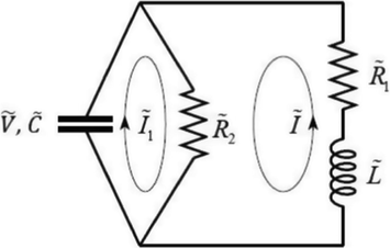
Electric circuit.
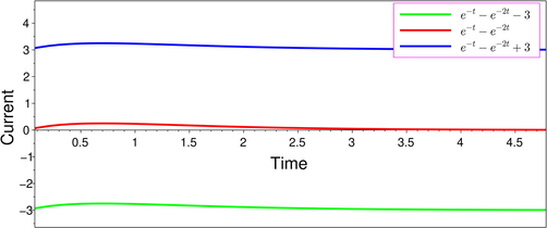
Current
for
hours.
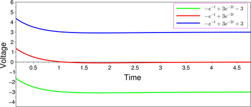
Voltage
for
hours.
The given system is modeled as a system of interval linear differential equations as
The interval matrix corresponds to the given system of interval linear differential equations (1) is
By applying the proposed pairing techniques, the interval eigenvalues of are and and the corresponding normalized interval eigenvectors are and respectively.
The solution of the given system of interval linear differential equations (1) is
Suppose that initially the voltage across
and loop current through
are approximately
and
respectively, we have the initial conditions
and
. Applying these initial conditions in equation (2), we get
The above example refers to a system of interval linear differential equations arrived at based on the premise that the entries are uncertain which explains the system of interval linear differential equations which is solved.
With this choice of initial conditions and , our solution shows that as time progresses the capacitor discharges exponentially quickly through the circuit. In case the entries are precisely known, then the above solution automatically transforms to the solution of the crisp system of linear differential equations if we replace intervals in the solution by their corresponding mid points.
6 Conclusion
On the collection of all closed intervals in , a relation is defined which turns out to be an equivalence relation on . The collection of all equivalence classes under the defined equivalence relation is a field E which is isomorphic to . This field E in turn induces a vector space over E which is a finite dimensional vector space over E for . A whole gamut of ideas which are available in classical linear algebra can now be applied to over E including canonicalization of interval matrices to Diagonal form, Jordan form and Rational form. We can extend this study to Bilinear and Quadratic forms also and investigate some interesting applications of these forms.
In over E, we are able to obtain unique eigenvalues and normalized eigenvectors of interval matrices as in the classical case. We have provided the methodology for obtaining the eigenvalues and normalized eigenvectors of interval matrices with two suitable examples. The distinct advantage of the Field and Vector space structure introduced in this paper guarantees the applicability of celebrated theorems in classical linear algebra to interval linear algebra. By applying the proposed pairing techniques, we also discussed a real life example on electric circuit theory under uncertain environment which is modelled as a system of interval linear differential equations. Numerical examples are provided to illustrate the theory developed in this paper.
Declaration of Competing Interest
The authors declare that they have no known competing financial interests or personal relationships that could have appeared to influence the work reported in this paper.
References
- Introduction to Interval Computations (first ed.). New York: Academic Press; 1983.
- The Interval Eigenvalue Problem. ZAMM J. Appl. Mathe. Mech.. 1991;71(1):61-64.
- [CrossRef] [Google Scholar]
- On Arithmetic Operations of Interval Numbers. Int. J. Uncertainty, Fuzziness Knowledge Based Syst.. 2005;13(6):619-631.
- [CrossRef] [Google Scholar]
- On some properties of interval matrices. Int. J. Comput. Mathe. Sci.. 2007;1(1):35-42.
- [Google Scholar]
- Strongly universal and weak interval eigenvectors in max-plus algebra. Mathematics. 2020;8(8):1348.
- [CrossRef] [Google Scholar]
- Interval arithmetic in matrix computations. Part 2, SIAM. J. Num. Anal.. 1967;4(1):1-9.
- [Google Scholar]
- On the solution of linear algebraic equations with interval coefficients. Linear Algebra Appl.. 1969;2:153-165.
- [Google Scholar]
- Bounding the solution of interval linear Equations. SIAM. J. Num. Anal.. 1992;29(5):1493-1503.
- [Google Scholar]
- Global Optimization Using Interval Analysis (second ed.). New York: Marcel Dekker; 2004.
- The extreme eigenvalues and stability of real symmetric interval matrices. IEEE Trans. Automat. Control. 1992;37(4):532-535.
- [Google Scholar]
- Applied Interval Analysis (first ed.). London: Springer-Verlag; 2003.
- Outer interval solution of the eigenvalue problem under general form parametric dependencies. Reliab. Comput.. 2006;12(2):121-140.
- [Google Scholar]
- Computing eigenvalue bounds of structures with uncertain-but-non-random parameters by a method based on perturbation theory. Comm. Numer. Methods Engrg.. 2007;23(11):973-982.
- [Google Scholar]
- An interval-matrix branch and-bound algorithm for bounding eigenvalues. Optim. Methods Softw.. 2017;32(4):872-891.
- [CrossRef] [Google Scholar]
- Interval Methods for Systems of Equations (first ed.). Cambridge: Cambridge University Press; 1990.
- Linear algebra in the vector space of intervals. arXiv math. 2010;1:1-11. doi:1006.5311
- [Google Scholar]
- Bounds of eigenvalues for structures with an interval description of uncertain-but-non-random parameters. Chaos Solitons Fractals.. 1996;7(3):425-434.
- [Google Scholar]
- An approximate method for the standard interval eigenvalue problem of real non-symmetric interval matrices. Comm. Numer. Methods Engrg.. 2001;17(4):239-251.
- [Google Scholar]
- Solution theorems for the standard eigenvalue problem of structures with uncertain-but-bounded parameters. J. Sound Vib.. 2005;282(1–2):381-399.
- [Google Scholar]
- Eigenvalue bounds of structures with uncertain-but-bounded parameters. J. Sound Vib.. 2005;282:297-312.
- [Google Scholar]
- Theory and Methodology: On comparing interval numbers. Eur. J. Oper. Res.. 2000;127(1):28-43.
- [CrossRef] [Google Scholar]
- eigenvalues of Interval Matrix. Am. J. Appl. Math. Comput.. 2021;1(4):6-11.
- [CrossRef] [Google Scholar]
- Introduction to Linear Algebra (third ed.). Wellesley-Cambridge Press; 2003.
- Eigenvalues bounds for symmetric interval matrices. Int. J. Comput. Sci. Mathe.. 2015;6(4):311-322.
- [CrossRef] [Google Scholar]
- Theory of an interval algebra and its application to numerical analysis. Japan J. Indust. Appl. Math.. 2009;26:125-143.
- [Google Scholar]
- A simple method for error bounds of eigenvalues of symmetric matrices. Linear Algebra Appl.. 2001;324:227-234.
- [Google Scholar]
- An evolution strategy method for computing eigenvalue bounds of interval matrices. Appl. Math. Comput.. 2008;196(1):257-265.
- [Google Scholar]


