

Identification of Preisach hysteresis model parameters using genetic algorithms
⁎Corresponding author. hmarouani@ksu.edu.sa (H. Marouani),
-
Received: ,
Accepted: ,
This article was originally published by Elsevier and was migrated to Scientific Scholar after the change of Publisher.
Peer review under responsibility of King Saud University.
Abstract
Preisach model is widely used to characterize ferromagnetic material’s hysteresis. Thus, it is necessary to identify its parameters in order to complete magnetic hysteresis modeling successfully. In this paper, a stochastic identification method, Genetic algorithm, is implemented. The procedure consists of the minimization of the error between measurements and program results. Obtained results are compared with the classical nonlinear least square identification method and experimental hysteresis of a fully-process non oriented Fe-3 wt%Si steel sheet.
Keywords
Ferromagnetic materials
Genetic algorithm
Magnetic hysteresis modeling
Parameters identification
Preisach model

1 Introduction
Magnetic materials are widely used in many engineering applications like shape memory alloy, piezoelectric, piezoceramic, magnetostrictive, and electromechanical actuators. Magnetic field H (A/m), magnetization M (A/m), magnetic induction B (T), the susceptibility χ (dimensionless) and permeability µ (H/m) are some of the primary magnetic parameters. The magnetic behavior and properties of a material can be learned by studying its hysteresis loop. A hysteresis loop shows the relationship between induced magnetic flux (B) and magnetic field (H).
In the past, several efforts have been made to develop different types of static hysteresis model. The classical Rayleigh model of scalar ferromagnetism (Lord, 1887) represents the H-M relation by a Prandtl-Ishlinksil model of play-type. This model is valid for small fields and it is fully determined by four experimental parameters (saturation magnetic field Hs, saturation flux density Bs, remanence flux Br and frequency f). The Fröhlich model (Frolich, 1881) is more adapted for the low hysteresis loss materials and is fully determined by four experimental parameters (Hs, coercitivity Hc, Bs and Br). Despite their simplicity, these models have limited applicability as they are specific to a particular variety of magnetic materials. The Langevin’s models are more accurate as they describe ferromagnetic material’s magnetization more accurately. The best known is the model of Jiles and Atherton (1986). It is a physical model of magnetic hysteresis and represents the magnetization M as a combination of a reversible component Mrev which results from the bending of the domain wall (Bloch walls) in the magnetization process and an irreversible one Mirr which corresponds to the domain wall displacement. The implementation of Jiles-Atherton uses five parameters (4 numericals and one experimental). The identification of these parameters is based on an iterative procedure (Jiles et al., 1992) which may introduce convergence problems. Moreover, it is very sensitive to initial values of parameters chosen as starting point for the optimization (Marion, 2008).
One of the most famous phenomenological hysteresis models is the Preisach model (Preisach, 1935). The popularity of this model is linked to the inventive technique of handling the contribution of infinite number of hysteresis operators with the Preisach triangle, the staircase line and the Everett function (Mayergoyz, 1991). It is much appropriate for numerical implementation. Currently, Preisach model includes similar scalar and vector hysteresis models, like the product model (Kádár, 1987), the moving model (Della Torre et al., 1994) or the Prandtl–Ishlinskii model (Hassani et al., 2014). Depending on the used distribution function, the classical Preisach model is completely determined by 5 parameters: two of them are experimentally deduced (Hs, Ms) and the remaining are numerically identified.
In order to generate the magnetization process for a given magnetic material, it is necessary to identify the Preisach parameters and evaluate its performances with regard to experimental data. There are many solving algorithms, which are mainly classified into two groups: Deterministic methods and stochastic ones. Deterministic methods are rarely used as they are based on the resolution of the gradient of the objective function. While, stochastic methods can be adapted to different forms of problems. They are based on a random evolution and require a lot of evaluation of the objective function to constantly end up guessing the optimum. Among these stochastic methods, the most widely used for magnetic domain are neural network (Zakerzadeh et al., 2011), genetic algorithm GA (Anh and Kha, 2008; Belkebir et al., 2009), particle swarm optimization (PSO) and nonlinear least squares method (Levenberg, 1944; Marquardt, 1963).
This paper describes an approach of Preisach parameter identification using GA. The proposed modeling method has achieved significant improvements in both accuracy and computation time, compared to the nonlinear least square identification method. The proposed approach can be applied to identify any type of hysteresis models. To demonstrate the efficiency of the proposed model, experimental results on hysteresis of a fully-process non oriented Fe-3 wt%Si steel sheet were provided and compared.
2 Classical Preisach model
The Preisach analysis (Preisach, 1935; Mayergoyz, 1991), mainly used for describing static magnetic behavior for ferroelectric and ferromagnetic materials, has been used to model iron-silicon films, piezoelectrical materials, super elastic response of Shape Memory Alloys for seismic dampers and arterial stents and also thermal effects on magnetic behavior (Quondam et al., 2016).
The magnetic state of the material is represented by magnetic entities (hysterons) having two possible saturation states M = 1 and M = −1, as shown in Fig. 1.
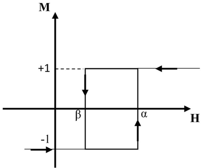
- Preisach elemental operator.
where,
The distribution of the elementary cycles defines the Preisach distribution function is expressed by (1).
The Preisach density is defined in the domain
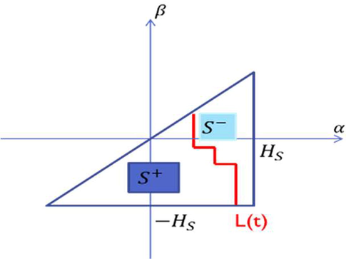
- Preisach triangle.
Indeed, for each t time of magnetization, the Preisach plane {S} is divided into two subdomains S+ and S− separated by a line L(t). This boundary line, with its stairway shape, generates the magnetic hysteresis. Actually, the vertical portions result from increasing excitation field values and the horizontal portions result from decreasing values of this field. It is generally described by two particular points; the starting point (α = Hs, β = −Hs) and the ending point (α = β = H(t)) which is located on the line α = β.
Different methods for identifying the distribution function have been developed. They can be identified using numerical approaches (Mayergoyz, 1991; Rousseau et al., 1997; Everett, 1955; Ben Abou et al., 2003) or using analytical approaches (Preisach, 1935).
The Lorentz Modified Function LMF is set by the coercitivity Hc, a regulator coefficient k and two parameters a and b. The distribution function by LMF is then given by (2):
Then, the total magnetization M(t) is expressed by (3)
3 Genetic algorithms
Genetic algorithms are stochastic algorithms. They consist on evolutionary optimization based on genetic mechanism and evolution of species of Darwin in 1960 with concepts like ‘mutation’, ‘crossing over’, ‘survival of the best individual’, ‘natural selection’… (Holland, 1975; Goldberg, 1989). Generally, the GA attempts to converge to the optimal solution by creating new individuals from an initial population according to a random process and the population progresses by successive generations recombining the best solutions together. Particularly, the GA works with ‘parameters coding’. Once genes codified, the identification process begins and follows the schematic presented in Fig. 3; first, an initial set of individuals that represents a solution of the considered problem is generated. Each individual is evaluated on its performance with respect to the fitness function imposed. The individual follows a selection process where the best (fittest) survives and selected to carry on the regeneration and others disappear. Parents exchange their genetic information randomly to produce innovative child population by crossover and mutation selected operators. The parents are then replaced in the population by the children to keep the population size stable.
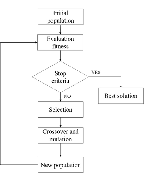
- Flow diagram of the GA.
This reproduction (Selection, crossover and mutation) is repeated and takes place with a probability of crossover (Pc) and probability of mutation (Pm), and it is again subjected to an evaluation of the relevance of the solution until the solution tends to the global optimum in a fixed iteration number.
In order to test the success of the model, several statistical criteria can be used. We can note ME (mean error), RMSE (root mean square error), R2 (coefficient of determination) and MAPE (mean absolute percentage error) which are based on comparing the estimated variables with the original one. They are expressed as follows (Hosseini et al., 2016):
The major ending criteria is the satisfaction of the imposed fitness value (error between experimental data and pretended ones). Then, the best fit time evolution is the second condition. If the parameter remains considerably unchanged after five consecutive iterations, then it should be a stop criterion (Consolo et al., 2006). Finally, the third criterion characterizes the number of population or generations initially fixed.
The benefit of GA is that they are suitable for complex problems. They are applied to functions with great number of parameters. In addition, GA is one of the most practical methods as it does not depend on the choice of the initial population. However, it requires many evaluations of the objective function to achieve the global minimum as it does not converge quickly. Several researchers have used the GA in their optimization studies and identification of parameters of magnetic models (Belkebir et al., 2009; Quondam et al., 2016; Wilson et al., 2001; Salvini and Fulginei, 2002; Che-Hang and Guangjun, 2007). All these studies have shown a considerable reliability of this algorithm.
4 Magnetic measurements test apparatus
Various magnetic measurement systems have been developed for different applications, such as magnetic behavior under mechanical stress and/or thermal modeling of magnetic components. The used magnetic experimental measurements test apparatus (Fig. 4) was validated by several experimental studies (Matsubara et al., 1989; Iordache et al., 2003). It consists of two U ferrite cores (Philips U100/57/25-3C90, MnZn material) maintained in contact with the sample close the magnetic circuit. Primary windings are wound on the central limbs of the yokes and secondary winding surround the specimen. This double-yoke arrangement leads to better homogeneous distribution of the magnetic field in the measurement zone, moreover it minimizes the negative effects of the overhang and of the eddy currents on the measurements accuracy.
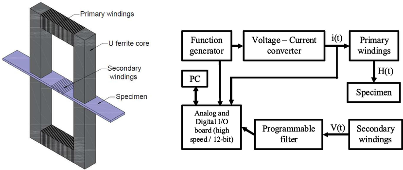
- Block diagram of the magnetic measurement test apparatus.
The magnetizing current waveform is controlled by a function generator and an operational amplifier. The voltage V(t) represents the direct output of the secondary coil and i(t) the input magnetizing current.
The magnetic field is estimated according to the IEC method (IEC, 1992) by:
The magnetic flux ΦS detected by the secondary winding is the sum of the flux experienced by the ferromagnetic specimen ΦSample and the magnetic flux in the air between the secondary winding and the specimen Φair:
The Faraday’s law requires that the secondary voltage V(t) on the secondary coil is proportional to the variation of the magnetic flux as:
The magnetic induction B(t) is calculated by integrating the secondary voltage V(t) with respect to Faraday’s law (13):
The used sample is a fully-process non oriented Fe-3 wt%Si steel sheet of 0.35 mm thick. The specimen is strips 20 mm wide and 250 mm long cut out in the rolling direction and vacuum annealed at 720 °C for 2 h in order to eliminate the residual stresses which originate from the manufacturing process (Hubert, 1998). Fig. 5 Shows the experimental obtained hysteresis.
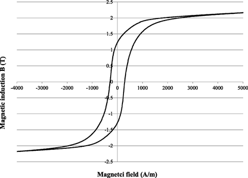
- Experimental hysteresis of a Fe-3 wt%Si steel.
5 Results and discussion
In this section, we investigate the ability of GA to identify the static Preisach model’s parameters that ensure reproducing the measured hysteresis curve of the Fe-3 wt%Si material. A comparative study is developed between GA and non-linear least square method (LSQ) in order to spot the more accurate. The identification procedures are established according to the following diagrams (Figs. 6 and 7) and are based on the minimization of two kinds of errors: the mean squared error and the percentage error described by Eqs. (14) and (15) respectively.
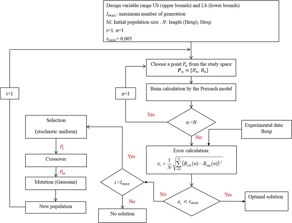
- Flow diagram of the used GA method (using ε1).
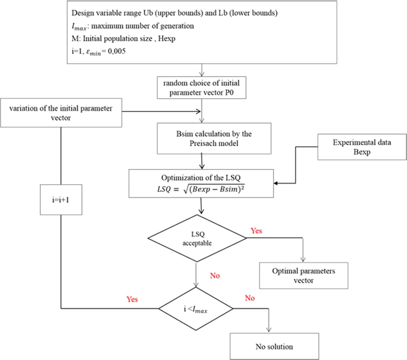
- Flow diagram of the LSQ method (using ε1).
Concerning the GA approach, the GA Matlab toolbox is used. The evaluation is carried out for an initial population of 20 individuals and 200 iterations. The crossover probability Pc and the mutation probability Pm are taken respectively equal to 0.8 and 0.2. Minimum and maximum expected values for the five Preisach parameters {a, b, k, Hs, Hc} are respectively {0, 0.3, 1000, 3500, 380} and {0.5, 1, 1500, 4500, 500}. Once the initial population is created, the Preisach model calculates the magnetic induction, which is then evaluated using the objective function (ε1 or ε2). The fitting results between measured and simulated values are provided at each run and compared to the major stop criterion εmin (=0.05). If convergence is not succeeded, the algorithm creates a new population by applying genetic operators (crossover and mutation). This new population is also evaluated and the process is repeated until convergence is reached.
Concerning the LSQ method, it consists on an iterative improvement of parameter values in order to reduce the sum of the squares of the errors between the function to be calculated and the measured data points. For this purpose, it requires an initial guess for the parameters to be estimated. So, we chose randomly the values a = 0.1, b = 0.75, k = 1200, Hs = 4400 and Hc = 420 for the initial guess. If the LSQ error is ‘acceptable’, the program ends and returns the optimal parameters. Otherwise, the algorithm resumes calculation for another initial parameters vector until 200 iterations.
According to the symmetry of the hysteresis, we just use the experimental half upstroke of the major loop for the identification process. The results of the optimization for the two methods for the conditions already mentioned are summarized in the following Table 1. The obtained curves using these identified parameters are shown in Fig. 8.
| Method | Error | Execution time (min) | Parameters | |||||
|---|---|---|---|---|---|---|---|---|
| ε1 (T) | ε2 (%) | a | b | k | Hs | Hc | ||
| GA | 0.026 | 0.53 | 40 | 0.2 | 0.7 | 1057 | 4044 | 444 |
| LSQ | 0.039 | 5.05 | 5 | 0.2 | 0.6 | 1000 | 3500 | 435 |
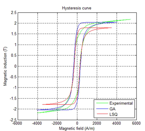
- Comparison of simulated cycles by GA and LSQ methods and experimental major cycle.
GA error ε1 evolution is shown in Fig. 9. The random choice of the initial population leads to a high value of the error. The creation of a new population by selecting individuals that have the better fitness value from the previous population improves drastically the error. For GA implementation, even if the fitness value εmin is not reached, and in case of the best individual of the population remains unchanged for a given number of generations (30), the algorithm converges. The obtained final solution is the optimal one. Fig. 9. Shows that GA converges at the 78th generation with a final error ε1 equal to 0.024 T.
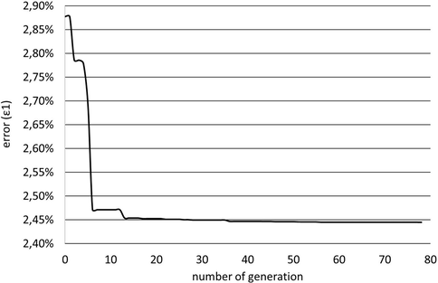
- Error evolution.
GA is based on a random choice of the initial population. Thus, we have different optimal points for the same upper and lower boundaries of designed parameters. Table 2 shows the results of five consecutives identifications. Identified half upstroke of the major loop are plotted on Fig. 10.
| Test | Error | Parameters | |||||
|---|---|---|---|---|---|---|---|
| ε1 (T) | ε2 (%) | a | b | k | Hs | Hc | |
| 1 | 0.020 | 0.35 | 0.3 | 0.4 | 1038 | 3854 | 401 |
| 2 | 0.021 | 0.51 | 0.3 | 0.55 | 1000 | 3786 | 398 |
| 3 | 0.025 | 0.99 | 0.2 | 0.7 | 1224 | 3815 | 412 |
| 4 | 0.023 | 0.49 | 0.2 | 0.4 | 1323 | 3913 | 426 |
| 5 | 0.024 | 0.640 | 0.2 | 0.7 | 1205.5 | 3886 | 425 |
| Average | 0.0225 ± 0.0025 | 0.67 ± 0.32 | 0.25 ± 0.05 | 0.55 ± 0.15 | 1161.5 ± 161.5 | 3850 ± 64 | 412 ± 14 |
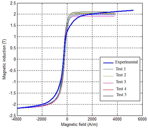
- Comparison of optimization results by GA and the experimental branch.
According to the sensitivity tests, we note that all the tests give errors less than 0.03 for ε1 and less than 1% for ε2. The parameter values are closely identical and gives superimposed curves. We note also that a strong dependency of the five model parameters a, b, k, Hm and Hc is existing.
6 Conclusion
In this paper we have proven how the static Preisach model’s parameters have been efficiently determined from limited set of experimental data (major loop) by the genetic algorithm approach and the non-linear least square method based on the Levenberg Marquardt algorithm. The results reached from the GA method are in a good agreement with the measures within an error of one percent and it produces the nearest cycle to the experimental reference one. So, it is more efficacious than the LSQ approach. Nevertheless, to prevent premature convergence and guarantee solution accuracy, the GA requires a large population size. Thus, a large population size usually demands more generations and consequently more computation time, which is a major weakness of this method.
Acknowledgement
The authors would like to extend their sincere appreciation to the Deanship of Scientific Research at King Saud University (Riyadh) for its funding of this research through the Research Group No RG-1439/007.
References
- Modeling and control of shape memory alloy actuators using Preisach model, genetic algorithm and fuzzy logic. J. Mech. Sci. Technol.. 2008;20(5):636-642.
- [Google Scholar]
- Identification et optimisation par algorithmes génétiques des paramètres du modèle de l’hystérésis magnétique de Chua. Revue des sciences et de la technologie. 2009;1(1)
- [Google Scholar]
- Comparison of Preisach and Jiles-Atherton models to take into account hysteresis phenomenon for finite element analysis. J. Magn. Magn. Mater.. 2003;261:139-160.
- [Google Scholar]
- Hysteresis identification and compensation using a genetic algorithm with adaptive search space. Mechatronics. 2007;17:391-402.
- [Google Scholar]
- Removing numerical instabilities in the Preisach model identification using genetic algorithms. Physica B. 2006;372:91-96.
- [Google Scholar]
- Modeling magnetic materials with the complete moving hysteresis model. J. Magn. Magn. Mater. 1994;133(1–3):6-10.
- [Google Scholar]
- A general approach to hysteresis part 4: an alternative formulation of the domain model. Trans. Faraday Soc. 1955;51:1551-1557.
- [Google Scholar]
- Investigations of dynamoelectric machines and electric power transmission and theoretical conclusions therefrom. Electrotech Z.. 1881;2:134-141.
- [Google Scholar]
- Genetic Algorithms in Search. Optimization and Machine Learning: Addison-Wesley; 1989.
- A survey on hysteresis modeling, identification and control. Mech. Syst. Signal Process.. 2014;49:209-233.
- [Google Scholar]
- Adaptation in Natural and Artificial Systems. A Bradford Book: The MIT Press, Cambridge, MA; 1975.
- Estimation of soil mechanical resistance parameter by using particle swarm optimization, genetic algorithm and multiple regression methods. Soil Tillage Res.. 2016;157:32-42.
- [Google Scholar]
- Doctorat thesis. France: Universite de Technologiede Compiegne; 1998.
- IEC (International Electrotechnical Commission), Magnetic materials-Part3: Methods of Measurements of the Magnetic Properties of Magnetic Sheet and Strip by Means of a Single Sheet Tester, IEC 404-3, 1992, pp. 1–35.
- Magnetic behaviour versus tensile deformation mechanisms in a non-oriented Fe–(3 wt.%)Si steel. Mater. Sci. Eng., A. 2003;359(1–2):62-74.
- [Google Scholar]
- Numerical determination of hysteresis parameters for the modeling of magnetic properties using the theory of ferromagnetic hysteresis. IEEE Trans. Magn. 1992:27-35.
- [Google Scholar]
- On the preisach function of ferromagnetic hysteresis. J. Appl. Phys.. 1987;61(8):4013-4015.
- [Google Scholar]
- A method for the solution of certain nonlinear problems in least squares. Quart. Appl. Math.. 1944;2:164-168.
- [Google Scholar]
- On the behavior of iron and steel under the operation of feeble magnetic forces. Phil. Mag.. 1887;23(142):225-245.
- [Google Scholar]
- Identification of Jiles-Atherton model parameters using Particle Swarm Optimization. IEEE Trans. Magn.. 2008;44:894-897.
- [Google Scholar]
- An algorithm for least –squares estimation of nonlinear parameters. J. Soc. Ind. Appl. Math.. 1963;11(2):431-441.
- [Google Scholar]
- Phys. Scr.. 1989;40:529.
- Mathematical Models of Hysteresis. New York: Springer-Verlag; 1991.
- Vector hysteresis model identification for iron-silicon thin films from micromagnetic simulations. Phys. B. 2016;486:97-100.
- [Google Scholar]
- Amélioration du modèle de Preisach. Application aux matériauxmagnétiquesdoux. J. Phys. III France. 1997;7:1717-1727.
- [Google Scholar]
- Genetic algorithms and neural networks generalizing the Jiles-Atherton model of static hysteresis for dynamic loops. IEEE Trans. Magn.. 2002;38(2):873-876.
- [Google Scholar]
- Optimizing the Jiles-Atherton model of hysteresis by a genetic algorithm. IEEE Trans. Magn.. 2001;37(2):989-993.
- [Google Scholar]
- Hysteresis nonlinearity identification using new Preisach model-based artificial neural network approach. J. Appl. Math.. 2011;2011
- [Google Scholar]


