Hybrid optimization assisted deep convolutional neural network for hardening prediction in steel

1.1 Literature review

2.1 Jominy test

“The Jominy end-quench test is the measure of the hardenability of steel, which is a measure of the capacity of the steel to harden in depth under a given set of conditions”. The heat handling can also be selected carefully for minimizing thermal stresses and disturbances when manufacturing components of different sizes. The hardness capacity of stones is important to choose the right combination of alloy steel. Hardness is dependent on the chemical steel mix, which has also been influenced, for example, the astonishing temperature, by prior manufacturing conditions. Not only is it important to be aware of the specific information obtained from the test, but also how the information obtained from the Jominy test is used to know the impacts of alloys on steels.

The diagrammatic representation and dimensions of the Jominy test are revealed in Fig. 1. A steel cylinder with a length of 100 mm and diameter of 25 mm is subjected to heating for a predetermined time within the austenitic area and it is quenched from its lower end with a standardized and controlled jet of water. The heat of water should lie between 15 and 25 °C. Based on the distance, the rate of cooling differs from 225 °C/s to 2 °C/s from the quenched end. Following the cooling process, the Jominy bar is refined in parallel to the axis of the cylinder on two sides. The outer region is grounded back for eliminating the issues related to decarburization and the hardening is evaluated from the quenched end at a certain period at this grounded surface. Thus, hardening could be measured at the cylinder axis in terms of distance from the quenched end. Fig. 2 shows the standard plot for depicting the hardenability of steel for varied distances from the quenched end.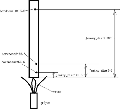

Close

Fig. 1

Diagrammatic Representation of Jominy test Considered.

Export to PPT

Close

Fig. 2

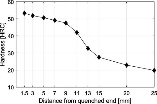
Hardenability of Jominy test.

Export to PPT

For the proposed framework, the input data mentioned are the chemical composition of steels such as “Carbon (C), Manganese (Mn), Silicon (Si), Phosphorus (P), Sulphur (S), Copper (Cu), Nickel (Ni), Chromium (Cr), Vanadium (V), Titanium (Ti), Niobium (Nb), Molybdenum (Mo), Aluminium (Al), Calcium (Ca), Lead (Pb), Tin (Sn), Antimony (Sb), Boron (B), Bismuth (Bi)”. Along with this, the distance from the quenched extremity is also considered. The formula of the respective chemical composition of the element is given in Table 2.

2.2 Framework of proposed hardenability prediction

The architecture of the proposed hardenability prediction model of the steel is demonstrated by Fig. 3. In this work, the chemical composition of steels such as C, Mn, Si, P, S, Cu, Ni, Cr, V, Ti, Nb, Mo, Alt, Ca, Als, Pb, Sn, Sb, B, W, H, Zr, Co, Bi, Zn, Ta, Se and F along with the distance parameters is given as inputs to DCNN framework. More particularly, to make the prediction more accurate, this work aims to optimize the convolutional layers of DCNN using the SL-DU algorithm, which ensures accurate prediction results.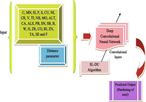

Close

Fig. 3

Diagrammatic illustration of the proposed framework.

Export to PPT

2.3 Deep convolutional neural networks

DCNNs [26] are CNNs that include numerous layers and it follows the hierarchical principle as given by Fig. 4. Following numerous Convolutional layers, deep CNNs usually include one or more wholly-connected layers, i.e., layers with denser weight matrix W. Apart from the input, spatial location is both quite inappropriate and partially lost and hence the local receptive regions of CNNs cannot be used. In case, if the classifier necessitates input quantity that behaves similarly to probabilities, the output phase can be a “softmax function” as given in Eq. (1), in which 1 denotes a column vector of ones.

Close

Fig. 4

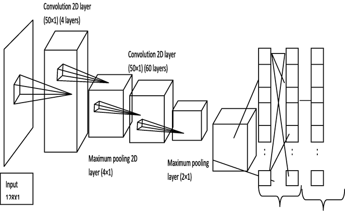
Pictorial demonstration of DCNN framework.

Export to PPT

In practice, the entire quantities are made positive by exponential, and normalization guarantees that the entries of $u$ adds up to 1. In general, the “softmax function” could be observed as a multidimensional generalization of the sigmoid function exploited in logistic regression (LR). This function is so-called “softmax” as one of the $x_i$ entries, e.g. $x_{i0}$ , is higher over the others, then $1^{T}exp\left(x\right)\approx exp\left(x_{i_0}\right)$ and hence Eq. (2) is formulated. The above function efficiently performs as an indicator among the highest entry in $x$ . Thus Eq. (3) is formed.

In short, DCNN carries out the below formulations mentioned in Eq. (4)-Eq. (7), in which the output activation function $f_x$ might be “softmax”, identity, or other function.

The matrix $W^{\left(q\right)}$ includes $F^{\left(q\right)}$ rows and $F^{\left(q-1\right)}+1$ columns with $F^{\left(0\right)}=F$ and $F^{\left(q\right)}$ for $q>0$ , which is equivalent to the output count in $q^{\mathit{th}}$ the layer. The initial $Q_c$ layers are convolution and the remaining ones are wholly connected.

3.1 Solution encoding and objective function

In the presented work, for better harden ability prediction of steel, it is planned to tune the optimal Convolutional layers $\left(Q_c\right)$ of DCNN. The solution encoding for the proposed prediction model is shown in Fig. 5, which $N_b$ represents the count of Convolutional layers in DCNN. Here, the objective function ( $\mathit{OF}$ ) of the presented work is defined in Eq. (8), where $\mathit{Err}$ denotes the error between actual and predicted value.

Close

Fig. 5

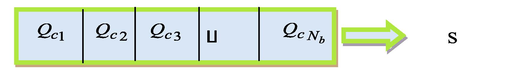
Solution encoding.

Export to PPT

3.2 Conventional dragonfly algorithm

The core inspiration of the DA model [25] is the swarming processes associated with the two main steps:(i) Exploration and (ii) Exploitation. Both phases are modeled as follows: as in Eq, the separation formula is evaluated. An error occurred (9), which $S_l$ reveals the $l^{\mathit{th}}$ , S indicates the location of the neighboring person, and N indicates the count of the people around him.

Alignment is measured as defined in Eq. (10), which $Q_l$ signifies the velocity of the $l^{\mathit{th}}$ neighboring individual. Also, the formulation for cohesion is given by Eq. (11), which $S_l$ specifies, the position of the $l^{\mathit{th}}$ neighboring individual $N_b$ symbolizes the neighbor count and $S$ signifies the position of the current individual. Attraction to a food resource is computed by Eq. (12), which $S^{+}$ corresponds to the position of the food source and $S$ signifies the current individual position.

Eq. (13) determines the distraction to an opponent, which $S^{-}$ describes the enemy’s position and $S$ denotes the present position of individuals. To update and carry out movements of dragonflies in a space of discovery, the evaluation of two vectors is a phase ( $\mathrm{\Delta }S$ ) and position ( $S$ ).

The step vector exposes the moving direction of the dragonfly, as computed in Eq. (14). Here, $C_i$ indicates the separation of $i^{\mathit{th}}$ individual, $q$ denotes the separation weight, $a$ denotes the alignment weight, $O$ signifies the $i^{\mathit{th}}$ individual cohesion, $c$ refers to cohesion weight, $B$ and $F_i$ points to alignment and food resource of $i^{\mathit{th}}$ individual respectively $f$ symbolizes food factor, $b$ corresponds to enemy factor, $w$ refers to the inertia weight, $E_i$ signifies enemy’s position of the $i^{\mathit{th}}$ individual and $\mathit{it}$ indicates iteration counter.

The position vectors are manipulated by Eq. (15) after the evaluation of the phase vector, where the latest version is shown.

It is important to travel around the discovery region where there are no neighboring solutions to boost the stochastic efficiency of the artificial floats. Under these conditions, the location of the dragonfly is updated by Eq. (16), in which the vector position dimension is represented and the current iteration is represented.

The Levy flight is evaluated by Eq. (17), which $\eta$ is a constant factor and $r_1$ $r_2$ is the random numbers that are lying among [0, 1]. Further, $\delta$ is computed using Eq. (18), in which $\mathrm{\Gamma }\left(x\right)=\left(x-1\right)$ . Algorithm 1 depicts the pseudo-code of the conventional DA model.

3.3 Conventional SLnO algorithm

SLnO [24] is a recent optimization approach that is developed based on the hunting behavior of sea lions. The major stages regarding the hunting behavior of sea lions are

• Tracing and chasing of prey by their whiskers.

• Pursuing and encircling the prey by calling the sea lions of their subgroups to join them.

• Attacking the prey.

3.4 Proposed Algorithm: SL-DU

For hardening prediction of the steel, this paper is designed to refine the Convolutionary layers of DCNN that can achieve a precise prediction. There is a suggestion for a new hybrid algorithm incorporating the ideas of DA and SLNO to resolve the limitations, such as poor convergence. In the traditional solution, DA is modified with levy according to Eq. The method of the hybrid algorithm is as follows: There was a mistake (16). In the proposed algorithm, the levy update of DA is evaluated by the position update of the SLnO algorithm. i.e. the levy update is as per Eq. (23) and the corresponding distance is computed using Eq. (22). The updated model is called the SL-DU model since it relies on a SLnO upgrade in DA. Algorithm 2 shows the pseudo-code of the SL-DU algorithm proposed. Fig. gives the representation of the flowchart (Fig. 6).

Close

Fig. 6

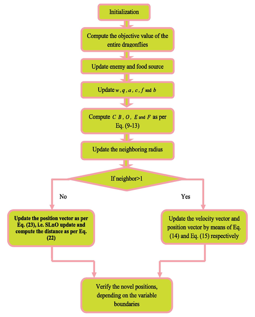
Flowchart of proposed SL-DU model.

Export to PPT

4.1 Simulation procedure

The adopted hardening prediction of steel was executed in MATLAB using the SL-DU model and the corresponding outcomes were attained. The process of experimentation for data collection is mentioned in the above section. Here, the performance of the presented technique was compared over the other conventional schemes like regression [27], MVR [28], ANN [29], and CNN [30] to error measures like MAE, MAPE, RMSRE, and R-value. The R-value was computed as per Eq. (24).

Further, To verify the work's results, statistical analytics was also performed. In the presented work, the analysis was carried out under two cases. Here, 321 records and 24 attributes were considered for experimentation (i.e. size of 321 × 24) and along with that, 10 values of distance (1.5, 3, 5, 7, 9, 11, 13, 15, 20, and 25) were also taken into account. Accordingly, each distance was added up with the attributes and thus, the size of the dataset turns out to be 321 × 25. Thus, ten sets of data were formed using ten values of distance. Under the first case, for all the ten sets of data, 70% was exploited for the training phase and the remaining 30% of data was exploited for the testing phase. Accordingly, the second case was carried out for five experimentations. During the 1st experimentation, the first two sets of data were exploited for the testing phase and the remaining eight sets of data were exploited for the training phase. Similarly, during the 2nd experimentation, the third set and fourth sets of data were exploited for the testing phase and the remaining datasets were exploited for the training phase. While carrying out 3rd experimentation, the fifth and sixth sets of data were exploited for the testing phase and the remaining datasets were exploited for the training phase. While performing the 4th experimentation, the seventh and eighth sets of data were exploited for the testing phase and the remaining datasets were exploited for the training phase, whereas, during 5th experimentation, the ninth and tenth sets of data were exploited for the testing phase and the remaining datasets were exploited for the training phase.

5.1 Analysis on Prediction

This section explains how much the mentioned methods correlate with the prediction accuracy. From the graphical representation (Fig S1 and S2), the x-axis declares the actual harden ability and the y-axis declares the predicted harden ability for varied distance values. Altogether, the graphs prove that the proposed method's predicted value is much closer to the actual value. However, conventional methods show their poor performance. In for an actual value of 0.94, the predicted harden ability output of the proposed is almost nearer to the actual value, whereas the values attained by the remaining methods scatter throughout the space. Similar results have been observed for all the distances. Thus the effectiveness of the proposed algorithm has been proved over other models.

5.2 Optimization Performance

The plots of the box are usually used to show details on the properties of the research conducted. Here, the analysis was carried out by plotting the fitness against varied iterations. Fig. S3 shows the optimization performance on the box plot for case 1. Since the goal or fitness function is to minimize errors, the plot needs to demonstrate that the proposed model progressively minimizes fitness. Fig S3 reveals the result for 25 iterations. As the iteration increases, the proposed model reveals gradual minimization of fitness. Thereby, at iteration 25, the least value is obtained that is in the range of 19 to 19.5.

5.3 Error Analysis

The error analysis of the proposed over traditional schemes is given by Table 3 on considering the overall values of distance. The error measures like MAE, MAPE, and RMSRE should be minimal for the adopted work, whereas the R-value should be higher to finalize precise prediction of the harden ability of steel. From Table 3, it is observed that the error value (MAE) obtained by the proposed model is linearly less than other models, which directly proves the betterment of the proposed model with precise prediction. Similarly, for MAPE, the least value 2.8297 is obtained by the proposed work, whereas the remaining models attain a higher value. The R-value evaluation is done as per Eq. (24), which should be higher when compared to other models. This is also proved by the proposed model with the utmost value of 0.99893.

Moreover, the analysis was held for the ten different distance values and the variation among the actual and predicted values during the testing phase are plotted in Tables S1–S4 concerning MAE, MAPE, RMSRE, and R-values respectively. From Tables S1–S4, the error measures are low for the presented method when evaluated over the traditional methods. Specifically, from Table S1, the MAE of the proposed scheme for distance 1.5 is 77.16%, 9.84%, 12.71%, and 23.36% better than the regression, MVR, ANN, and CNN. Also, from Table S2, the MAPE of the adopted scheme for distance 5 is 82.93%, 68.36%, 34.25%, and 9.64% superior to regression, MVR, ANN, and CNN models. From Table S3, the RMSRE of the suggested scheme is 90.29%, 42.65%, 57.1%, and 49.09% superior to regression, MVR, ANN, and CNN approach. Also, from Table S4, the R-value is higher for the adopted model, which is 21.75%, 2.87%, 0.63%, and 0.1% superior to regression, MVR, ANN, and CNN models Thus, the betterment of the adopted model is confirmed from the outcomes (Table S5 and S6).

5.4 Statistical Analysis

Since the meta-heuristic algorithms are intangible, the same outcome cannot be obtained. Thus, five times it is finished, and the best bad, middle, and standard deviation is defined. All the listed error measurements have been statistically evaluated. From the results, With decreased error behaviour, the presented plan achieved better performance than the other existing programs. More particularly, from Table S8, the mean of the proposed scheme for distance 1.5 is 77.16%, 9.84%, 12.71%, and 23.36% better than the regression, MVR, ANN, and CNN. Also, from Table S8, the standard deviation of the adopted scheme for distance 1.5 is 88.09%, 36.68%, 34.93%, and 8.49% better than the regression, MVR, ANN, and CNN models. Similarly, Table S9 summarizes the results under the median and worst-case scenario for varied distances. Thus, the predicting capability of the adopted scheme is proved to be efficient over the other traditional schemes.

5.5 Results analysis under case 2

Fig. S4 demonstrates the optimization performance on the box plot for case 2 by plotting the fitness against varied iterations. Here, the adopted work intends on error minimization and therefore, the plot should reveal a gradual minimization of fitness. The fitness is evaluated for 25 iterations and accordingly, a gradual minimization of fitness is attained by the presented model with an increase in the iteration.

References

- Prediction of radiation induced hardening of reactor pressure vessel steels using artificial neural networks. J. Nucl. Mater.. 2011;408(1):30-39.
- [Google Scholar]
- Non-destructive hardness prediction for 18CrNiMo7-6 steel based on feature selection and fusion of Magnetic Barkhausen Noise. NDT & E Int.. 2019;107:102138.
- [CrossRef] [Google Scholar]
- The numerical model prediction of phase components and stresses distributions in hardened tool steel for cold work. Int. J. Mech. Sci.. 2015;96-97:47-57.
- Modelling of anisotropic hardening behavior for the fracture prediction in high strength steel line pipes. Eng. Fract. Mech.. 2015;148:363-382.
- Using dragonfly algorithm for optimization of orthotropic infinite plates with a quasi-triangular cut-out. Eur. J. Mech. A/Solids. 2017;66:1-14.
- Physically based modeling, characterization and design of an induction hardening process for a new slurry pipeline steel. Mater. Des.. 2019;182:108047.
- Bio-inspired weighed quantum particle swarm optimization and smooth support vector machine ensembles for identification of abnormalities in medical data. SN Appl. Sci.. 2019;1(10):1-10.
- A novel architecture for next generation cellular network using opportunistic spectrum access scheme. J. Adv. Res. Dynam. Control Syst.. 2017;12:1388-1400.
- Prediction of irradiation hardening in austenitic stainless steels: Analytical and crystal plasticity studies. J. Nucl. Mater.. 2019;518:316-325.
- Multiscale modeling of crystal plasticity in Reactor Pressure Vessel steels: Prediction of irradiation hardening. J. Nucl. Mater.. 2019;514:128-138.
- Evaluation of ratcheting behaviour in cyclically stable steels through use of a combined kinematic-isotropic hardening rule and a genetic algorithm optimization technique. Int. J. Mech. Sci.. 2019;152:138-150.
- Prediction of hardness and deformation using a 3-D thermal analysis in laser hardening of AISI H13 tool steel. Appl. Therm. Eng.. 2017;121:951-962.
- Deep learning model for predicting hardness distribution in laser heat treatment of AISI H13 tool steel. Appl. Therm. Eng.. 2019;153:583-595.
- Prediction of flank wear by using back propagation neural network modeling when cutting hardened H-13 steel with chamfered and honed CBN tools. Int. J. Mach. Tools Manuf. 2002;42(2):287-297.
- Optimal stochastic gradient descent with multilayer perceptron based student's academic performance prediction model. Recent Adv. Comput. Sci. Commun. 2019
- Role of gender on academic performance based on different parameters: data from secondary school education. Data Brief. 2020;29:105257.
- Prediction of age hardening parameters for 17–4PH stainless steel by artificial neural network and genetic algorithm. Mater. Sci. Eng. A. 2016;675:147-152.
- VHCF properties and fatigue limit prediction of precipitation hardened 17–4PH stainless steel. Int. J. Fatigue. 2016;88:205-216.
- Deformation and fatigue behaviors of case-hardened steels in torsion: experiments and predictions. Int. J. Fatig.. 2009;31(8-9):1386-1396.
- Fatigue characteristics and fatigue limit prediction of an induction case hardened Cr–Mo steel alloy. Mater. Sci. Eng. A. 2003;361(1-2):15-22.
- Quantitative prediction of residual stress and hardness in case-hardened steel based on the Barkhausen noise measurement. NDT & E Int.. 2012;46:100-106.
- A taxonomy of deep convolutional neural nets for computer vision. Front. Robot. AI. 2016;2:36.
- Prediction of hypo eutectoid steel softening due to tempering phenomena in laser surface hardening. CIRP Ann.. 2008;57(1):209-212.
- Mixed mode I/II failure prediction of thin U-notched ductile steel plates with significant strain-hardening and large strain-to-failure: the Fictitious Material Concept. Eur. J. Mech. A/Solids. 2019;75:225-236.
- Prediction of the yield strength of a secondary-hardening steel. Acta Mater.. 2013;61(13):4939-4952.
- Variable amplitude fatigue behavior and life predictions of case-hardened steels. Int. J. Fatigue. 2010;32(7):1126-1135.
Appendix A
Supplementary data
Supplementary data to this article can be found online at https://doi.org/10.1016/j.jksus.2021.101453.
The following are the Supplementary data to this article: