

Translate this page into:
Homotopy perturbation transform method for pricing under pure diffusion models with affine coefficients
⁎Corresponding author. pindzaedson@yahoo.fr (Edson Pindza),
-
Received: ,
Accepted: ,
This article was originally published by Elsevier and was migrated to Scientific Scholar after the change of Publisher.
Peer review under responsibility of King Saud University.
Abstract
Most existing multivariate models in finance are based on diffusion models. These models typically lead to the need of solving systems of Riccati differential equations. In this paper, we introduce an efficient method for solving systems of stiff Riccati differential equations. In this technique, a combination of Laplace transform and homotopy perturbation methods is considered as an algorithm to the exact solution of the nonlinear Riccati equations. The resulting technique is applied to solving stiff diffusion model problems that include interest rates models as well as two and three-factor stochastic volatility models. We show that the present approach is relatively easy, efficient and highly accurate.
Keywords
Diffusion model
Interest rate
Stochastic volatility
Stiffness
Laplace transform
Homotopy perturbation method

1 Introduction
Stochastic processes have taken over the world of financial modelling. Starting with simple Geometric Brownian Motion well described by Bachelier (1900), to more sophisticated processes for better fitness and calibration of market fluctuations. A huge range of papers have considered Lévy processes as their driving force, they usually take the umbrella of jump diffusion process. Basically the state process follows a Brownian motion with drift for which a pure jump process, usually of Poisson type, is added on in order to accommodate abrupt changes in the market. In this work we restrict ourselves to pure diffusion processes for which the drift, the variance as well as the interest rate processes are all affine functions of ; we refer the reader to Eq. (2.4) in the next section for the explicit form. Duffie et al. (2000) present a general framework of diffusion processes under affine coefficients (also termed as affine models) then apply it to a two dimensional option pricing problem. These diffusion models have the advantage of providing tractability of closed form formula for a wide range of asset price such as fixed income securities: bonds, options and swaps. Technically, in dealing with these diffusion models we apply transforms that will result later in a system of ordinary differential equations of Riccati type that can be solved analytically or numerically in order to compute the asset price. In most cases, numerical methods using Fourier transform or inverse Laplace transform are needed to solve the integro-differential equation that arise thereof.
Various types of diffusion models have been introduced in the literature and used in different sectors. They differ in the model parameter while preserving some properties that are essential in asset price dynamics such as mean reversion.
In one-factor models the volatility process is a deterministic function of t, this includes the class of affine term structures that is encountered in interest rates and option pricing contexts, see Duffie (2005), Björk (2004), Black and Scholes (1973) and Merton (1974).
Heston (1993) introduces a two-factor model where the volatility is now stochastic, to accommodate the implied volatility smile encountered in the financial markets as shown by Kotzé et al. (2015). Bates (1996) extends the Heston model in adding a up jumps into the diffusion process to model a huge flux of information that can occur in the market.
Fang (2000) brings a three-factor model with jump diffusion process that looks quite stable. The model takes its roots from the Bates model to which an extra parameter is added: the long-term volatility, which is important for instruments like bonds that have long term maturity. Banks are often interested in this parameter. Christoffersen et al. (2009) consider a three-factor model with no jumps, but the state process is driven by a deterministic drift, plus two Brownian motions. However, as the number of factors increases one must expect the model to become more robust, but less realistic. In this paper we present a detailed framework of a class of asset prices whose pay-off at a future time (the maturity time) T is of the form where is of a pure diffusion type with affine coefficients. This class includes fixed income security prices. A quick overview of the pure diffusion with affine coefficients is provided together with an application on bond price in the context of single, two and three-factor models based on the Heston type. In other words, the volatility is considered to be stochastic. This Gives them a wider range of application. Bravo (2008) uses an affine process for pricing longevity bonds; Jang (2007) applies a two-factor affine process in insurance; Crosby (2008) uses it in pricing a class of exotic commodities and options in a multi-factor model.
In addition we introduce a modified form of homotopy perturbation and Laplace transform methods to value financial models of diffusion type with affine coefficients. These models lead to the need of solving systems of Riccati differential equations. Laplace transform method (LTM) alone is incapable of handling such equations, instead some variants of the LTM prove to better handle nonlinear differential equations. Among those variants we cite the Laplace decomposition algorithm (Khuri, 2001; Khan, 2009) and the H2LTM, (Fatoorehchi and Abolghasemi, 2016) which are obtained with the help of the Adomian decomposition and Adomian polynomials respectively. Another successful variant of LTM is obtained in coupling it with variation iteration methods. Alawad et al. (2013) used it to solve space–time fractional telegraphic equation as it allowed them to overcome the difficulty arising from finding Lagrange multipliers. LTM has also known great success when combined with differential transform methods on solving non–homogenous equations, see Alquran et al. (2012). On the other hand, the homotopy perturbation method is a combination of the classical perturbation technique and the homotopy technique whose origin is in topology , more on homotopy can be found in Hilton (1953), but not restricted to small parameters as it occurs with traditional perturbation methods. For example, the HPM requires neither small parameters nor linearisation, but only few iterations to obtain highly accurate solutions. The standard homotopy perturbation method was proposed by He (1999) as a powerful tool to approach various kinds of nonlinear problems. It can also be viewed as a special case of Homotopy Analysis Method (HAM) proposed by Liao (1992, 1997). For the past decade, many improvements on HAM have been introduced, one of it being the Homotopy Analysis Transform Method (HATM) which is basically a HAM coupled with a Laplace transform. The method is very powerful, fast converging and accurate. Recently, it has been applied in many different areas of science including fluid dynamics, wave theory (Kumar et al., 2014a, 2015b, 2016b), quantum physics, see Kumar (2014), and many more, with extension to fractional cases. Kumar et al. (2014c) applied this method on Volterra integral equation to obtain good quality results. Another improvement of HAM is obtained by coupling it with the Samudu transform which gives rise to the Homotopy Analysis Samudu Transform Method (HASTM), see Kumar and Sharma (2016); Kumar et al., 2016a for more details. Likewise, the Samudu transform has also been introduced in HPM to generate the Homotopy Perturbation Samudu Transform Method (HPSTM), see Singh et al. (2013); Singh et al., 2014b. Singh et al. (2014a) used the method successfully to get analytical and numerical solutions of nonlinear fractional equations found in the area of biological population model. Also, Kamdem (2014) proposed a generalised integral transform based on the homotopy perturbation method where various integral transforms were used. In this paper we are interested in the combination of the HPM with Laplace transform giving rise to the Homotopy Perturbation Transform Method (HPTM). The method has shown success already in obtaining solutions of the Navier–Stokes equations (Kumar et al., 2015a), gas dynamics equations coming from fluid dynamics in the case of fractional differential equation as explored by Kumar et al. (2012). The method has also shown success in solving KdV equations arising in wave theory (Goswami et al., 2016) as well as Fokker-Planck equations commonly found in solid-state physics (Kumar, 2013). Another useful application of the technique is found in Kumar et al. (2014b) in which the authors derive the price of a plain vanilla call option of European type under Black–Scholes model in the financial market.
This paper is structured as follows: Section 2 reviews the formalism of diffusion models with emphasis on the case with affine coefficients. In Section 3, we introduce the basic concept of homotopy perturbation transform method (HPTM). In Section 4, we describe the solution procedure of the HPTM for interest rate models, especially the two and three-factor stochastic volatility models. Finally, the conclusions are presented in Section 5.
2 Mathematical description of affine models
Consider the financial market model
where
is the set of all possible outcomes of the experiment known as the sample space,
is the set of all events, i.e. permissible combinations of outcomes,
is a map
which assigns a probability to each event,
is a natural filtration and
a risky underlying asset price process. The triplet
is defined as a probability space. Let
denote a
-Wiener process,
the volatility of the underlying asset,
the drift parameter. Suppose
satisfies the following stochastic differential equation
Under an equivalent martingale measure
, the price
at time t of a contingent claim that pays off
at maturity time
is given by
Let us consider an auxiliary process . For simplicity of notation, we may from time to time write to denote . Same for other variables as well. Applying the Ito’s differentiation we get
Under no-arbitrage conditions, the discounted pay-off
, must be martingale, meaning the drift part must be zero. That is,
In Affine framework as described by Cont and Tankov (2004), we consider
to be Affine in X. That is,
Theorem 2.1 see Duffie et al., 2000
Under technical conditions, if the pay-off function is chosen such that
then
is of the form
with
and
verifying the following Riccati equation
Given the pay-off a good candidate for the auxiliary process is where is the discounted pay-off. Under no arbitrage and the equivalent martingale measure martingale and . For any , we have the following
We can apply the above result on the auxiliary process to obtain
Using the Affine framework coupled with the fact that
we get
Implying,
Finally we have,
Eq. (2.7) together with initial condition (2.8) is a nonlinear system of ODE of Riccati type. In general, Riccati equations do not have analytical solutions, hence numerical methods have to be used. In addition, these equations have been reported to be stiff. Hence the use of explicit methods will require a high mesh refinement to produce acceptable solutions. This will result in an increase in the computational cost. In this article we propose a Laplace Transform Homotopy Perturbation method to circumvent the stiffness problem.
3 Basic idea of homotopy perturbation transform method
We first define the Laplace transform (LT) and its inverse transform, and list useful properties employed in this paper.
Laplace transform of
is denoted by
and is defined by the integral
The inverse Laplace transform is evaluated on a contour
, known as the Bromwich contour, as
The contour is chosen such that it encloses all the singularities of .
One useful property of LT for this paper is:
To illustrate the basic ideas of this method, let us consider the following system of nonlinear partial differential equations
In order to solve the system of differential Eq. (3.4) by means of the homotopy perturbation transform method, we construct the homotopy
, which satisfies the following
We apply the Laplace transform on both sides of the homotopy Eq. (3.8) to obtain
Using the differential property of the Laplace transform we have
By applying the inverse Laplace transform on both sides of (3.13), we have
Assuming that the solutions of Eq. (3.7) can be expressed as a power series of p
Then substituting Eq. (3.15) into Eq. (3.14), we get
Comparing coefficients of p with the same power leads to
Assuming that the initial approximation has the form
The utility of HPTM is shown by its applications on Affine diffusion problems.
4 Numerical experiments
4.1 Interest rate models
We first look at affine term structure models that are found in interest rate models (see Björk, 2004). Here the state process is the interest rate itself r following the dynamics: where and are deterministic functions of t. This suggests that the state process corresponds exactly to the interest rate . It is one dimensional, and as a result we have the following matching
For a zero coupon bond that pays 1 at maturity T, we see that its price at any time
prior to maturity is given by
with
and
satisfying the system of stiff ODEs of the form
We investigate numerical solutions of the system (4.1) by means of the HPTM. To this end we construct the following homotopy
Applying the Laplace transform on both sides of (4.2), we have
Using the differential property of the Laplace transform we have
By applying inverse the Laplace transform on both sides of Eq. (4.4) and after algebraic simplification we get
Suppose the solution of Eq. (4.2) to have the following form
We consider a particular case of the Vasicek model (see Björk, 2004). This model is obtained from Eq. (4.1) when the parameters are and . The exact solution of the Vasicek model was found to be of the form
The Taylor expansions of both and at about zero at order 6 is and
To obtain the numerical solution of the (4.1) for the Vasicek model, we assume
and
. Solving Eqs. (4.7)–(4.9) for
leads to the following result
The polynomials
and
are the same as the Taylor expansion obtained above for
and
, respectively. This means the limit of infinitely many terms (4.11) and (4.12) yields the exact solution (4.10). The accuracy of the scheme is measured using the following relative error
Table 1 illustrates the convergence of the HPTM. At
and as j increases from 4 to 10 the error in
decreases from order
to
and from
to
for
. At
and as j increases from 4 to 10 the error in
decreases from order
to
and from
to
for
.
1.19416E−5
9.66072E−5
1.55847E−3
4.36287E-3
1.30838E-2
5.29545E−8
8.61305E−7
3.53106E−5
1.39979E−4
6.10400E−4
2.72792E−9
8.86011E−8
9.02825E−6
4.98717E−5
3.08174E−4
3.1584E−12
2.05922E−10
5.30832E−8
4.14078E−7
3.70637E−6
3.84661E−13
4.88715E−11
3.13493E−8
3.40916E−7
4.32664E−6
8.13539E−17
2.92069E−14
4.63624E−11
7.1053E−10
1.30249E−8
1.11102E−14
1.99155E−15
7.16094E−11
1.53097E−9
3.98281E−8
1.91192E−16
5.38435E−16
2.64043E−14
7.95826E−13
2.98415E−11
Fig. 1 (a) shows that the exact and numerical solutions of Eq. (4.1) are in good agreement. The bond price behaviour as a function of and is captured in Fig. 1(b).
In this experiment, we consider the Cox-Ingerson-Ross (CIR) model (see Björk, 2004). This model is obtained from Eq. (4.1) when the parameters are and . The exact solution of this model is
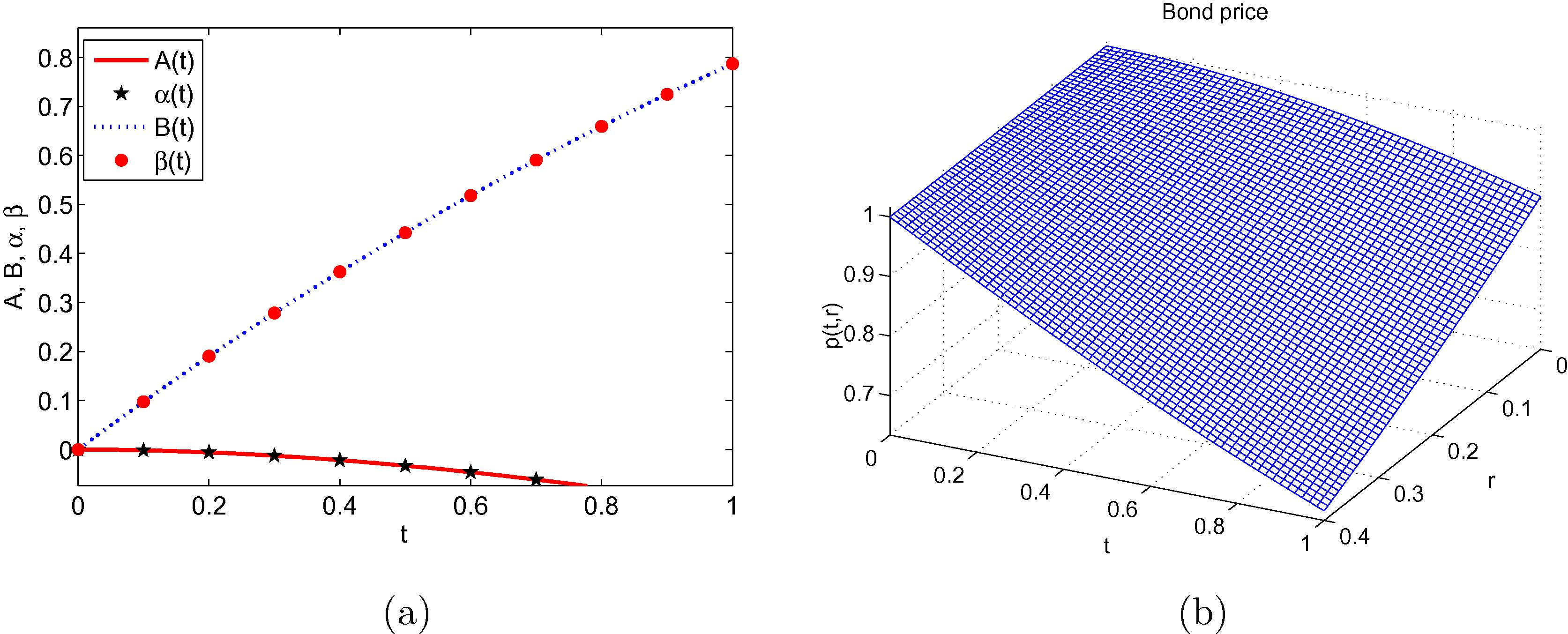
- (a) Exact and numerical solutions of 4.1 and (b) Bond price process for the Vasicek model when
and
at
.
Using the initial conditions and , we solve Eq. (4.1) for . Considering the bond that pay-off 1 at maturity implies . The solution computed using the HPTM at order is given by
Again we observe that the Taylor expansion and the solution of the CIR model computed by the HPTM are in good agreement. Table 2 records the error for different values of j and different values of
taken randomly. The same conclusion applies as to the Vasicek model, that the error decreases rapidly as
gets closer to 0. The bond price in terms of time to maturity
and the interest rate r is given by
1.43085E−5
1.16921E−4
4.02833E−4
9.74221E−4
1.9403E−3
4.95614E−7
8.31425E−6
4.40686E−5
1.45623E−4
3.71224E−4
1.07357E−10
5.13301E−9
5.16706E−8
2.71528E−7
9.93647E−7
2.00642E−10
1.30547E−8
1.51097E−7
8.62187E−7
3.33847E−6
2.68126E−12
1.90102E−10
3.28522E−9
2.49695E−8
1.20746E−7
1.28341E−13
3.43621E−11
9.14227E−10
9.47091E−9
5.84918E−8
1.22378E−12
7.96574E−13
5.11847E−12
7.03396E−11
5.42104E−10
7.29208 E−16
1.16398E−14
6.42225E−13
1.09941E−11
9.83115E−11
Fig. 2 shows the behaviour of the parameters
and
as well as the corresponding bond price (4.16) for
. Clearly, exact and numerical solutions are in good agreement.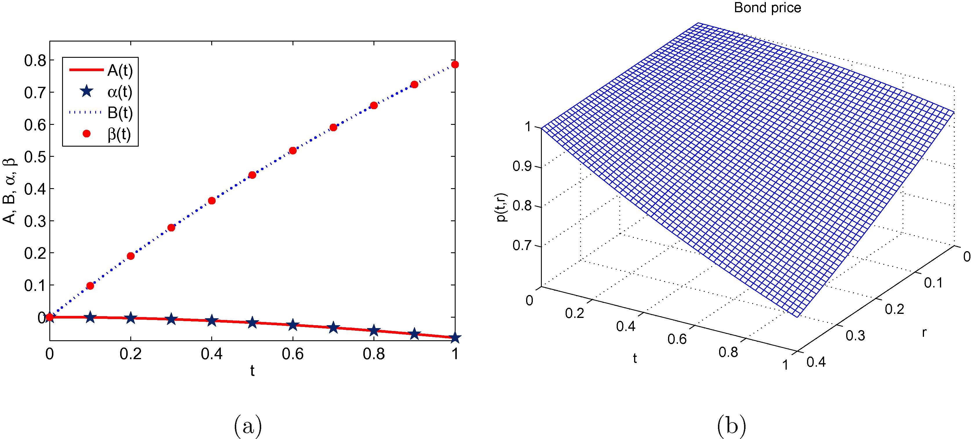
(a) Parameters
and
exact and approximate and (b) bond price behaviour for
.
4.2 Two-factor stochastic volatility model
One of the most well-known stochastic volatility models is the Heston model described by Duffie et al. (2000). Under constant interest rate r, the stock price has dynamics driven by
The stochastic differential Eq. (4.18) can be written as where and are independent processes. We consider in order to force the process to become Affine.
Let then . The state vector has linear dynamics and it is written as
Under the risk free equivalent martingale measure the process is governed by where i.e.
Referring to Affine settings, we see that
Eq. (2.3) is now two-dimensional and referred to as a two-factor model. By choosing the pay-off function in the form
Resulting in
The exact solution is given by
where
. To solve Eq. (4.23) by the use of the HPTM, we construct the following homotopy
Applying the Laplace transform on both sides of (4.24), we have
Using the differential property of the Laplace transform we have
By applying the inverse Laplace transform on both sides of (4.26) and after algebraic simplification, we have (see Fig. 4)
Suppose the solution of Eq. (4.27) to have the following form
Assuming and and solving the above equation for , we get the following graphs for and as is just constant and equal to u.
Here the parameters are chosen randomly as
. One can clearly see in Fig. 3 the quick convergence of the HPTM as
is small enough, but for
it is essential to increase the number j. The price at time
of the security that pays off
is given by
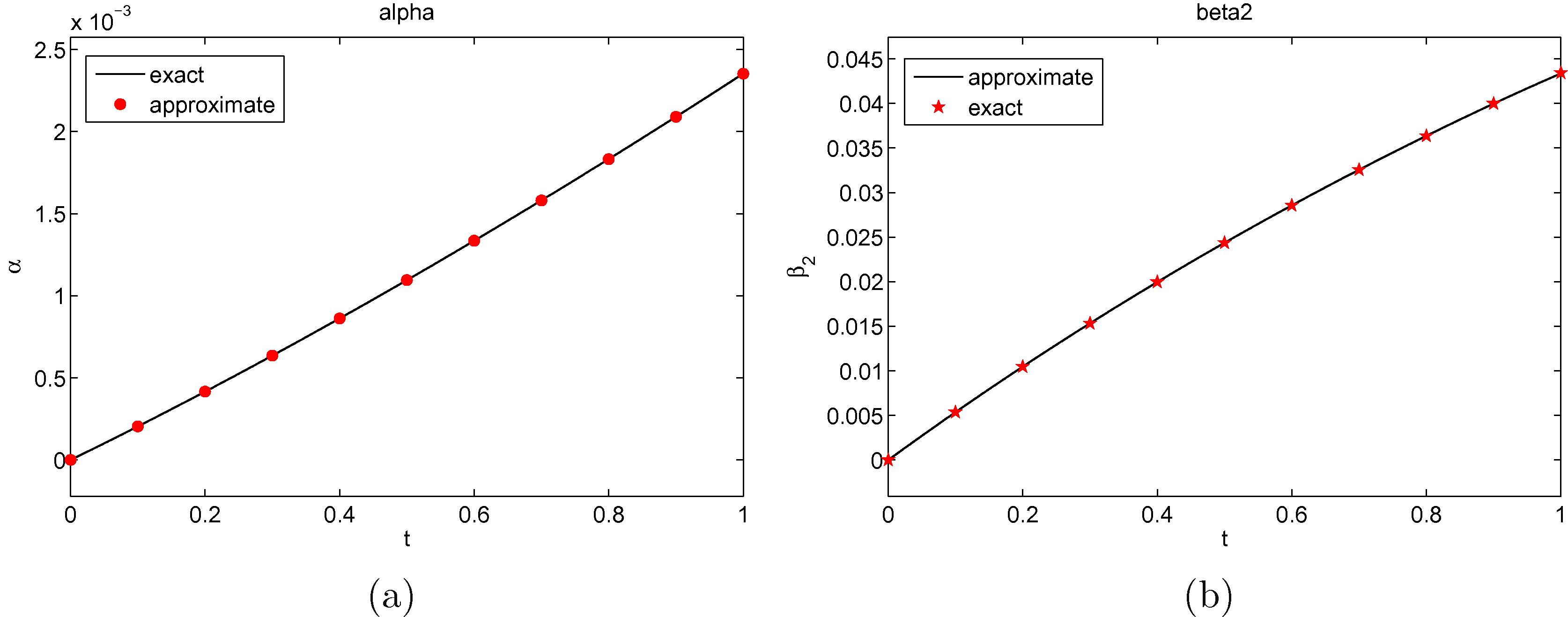
(a)
exact and approximate A for
and (b)
exact and its approximate C obtained for
.
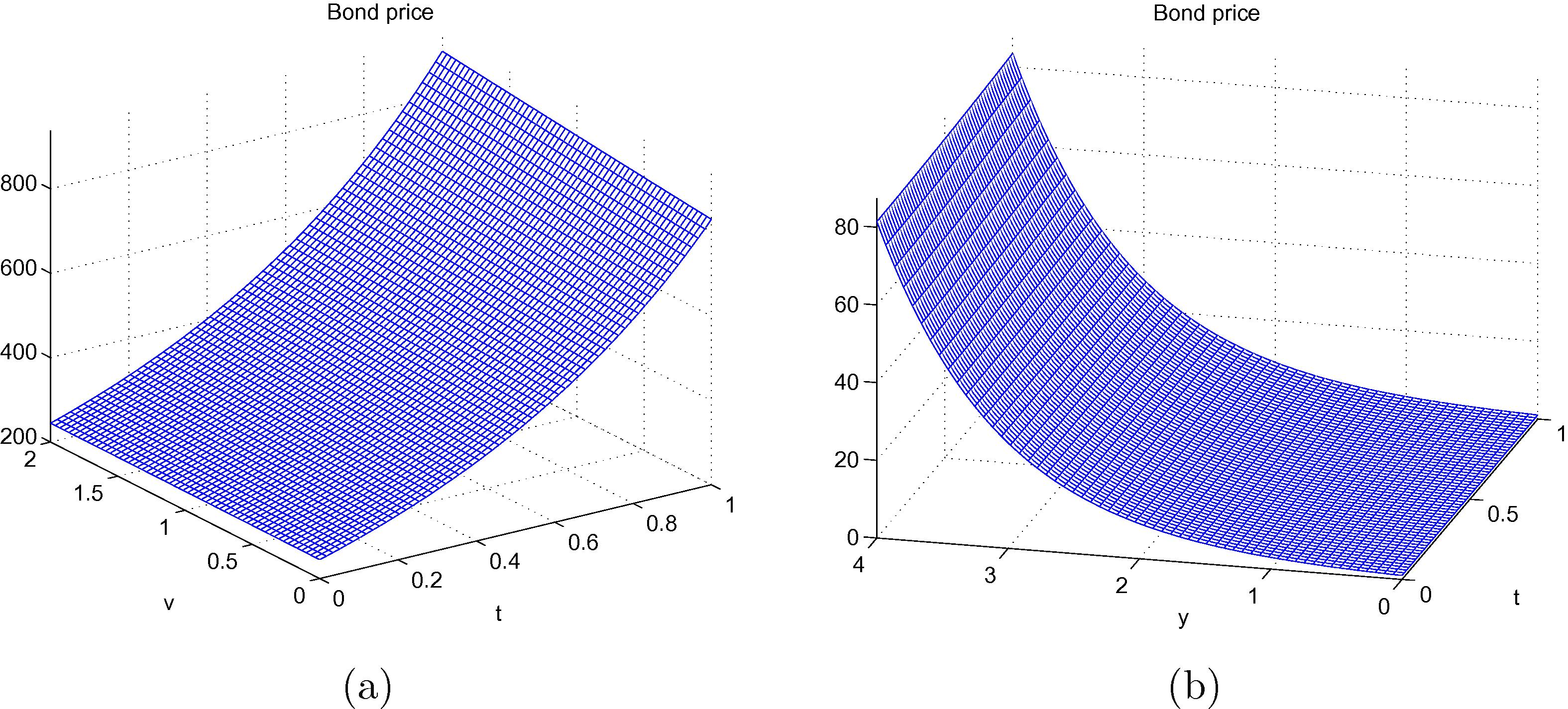
(a) Asset price behaviour with respect to
. (b) Asset price behaviour with respect to
.
If we consider with , we get the asset price behaviour sketched in Fig. 4(a). We can also view the asset price as a function of y and . For the sake of computation we consider v to be a polynomial of order 2 in , that is, we arbitrarily take . The resulting asset price behaviour is recorded in Fig. 4(b).
4.3 Three-factor stochastic volatility model
We consider the three-factors Heston model also considered by Duffie et al. (2000) where the state process
is the triplet
where
is the long-term volatility trend of the stock
. The state process dynamics under the equivalent martingale
is given by
We know the solution is given by Eq. (4.1) ie. with and satisfying and
After algebraic simplifications, we end up with the following system of ordinary differential equations of Riccati type
To solve Eq. (4.33) by the HPTM, we construct the following homotopy
Applying the Laplace transform on both sides of (4.34), we have
Using the differential property of the Laplace transform we have
By applying the inverse Laplace transform on both sides of (4.36) and after algebraic simplification we have
Suppose the solution of Eq. (4.36) to have the following form
Assuming
and
, we solve the above equation for
. For computational purpose we consider the following set of parameters:
. We run the HPTM for
. The results in Fig. 5 and Table 3 show that numerical solutions converge rapidly as j increases.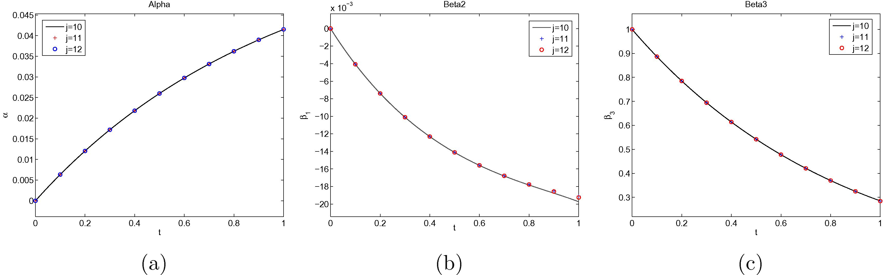
(a)
, (b)
and (c)
computed for
and
for
.
Defining the error function at order j to be
Table 3 records the errors in
at order 9. Note that
is constant since its derivative is 0.
9.44787E−10
2.88458E−7
8.75677E−6
1.02925E−4
7.17550E−4
2.92738E−8
1.00574E−5
3.40898E−4
4.44356E−3
3.42980E−2
5.24351E−10
3.73261E−7
2.00047E−5
3.72887E−4
3.91183E−3
5 Conclusion
In the present work, we proposed a combination of the Laplace transform method and the homotopy perturbation method to solve nonlinear systems of stiff Riccati differential equations arising in finance. We have discussed the methodology for the construction of these schemes and studied their performance on one, two and three-factor diffusion models with affine coefficients. The solution of these Riccati systems of equations by means of the homotopy perturbation transform method converges rapidly to the exact solution as the number of truncated term increases. The HPTM is an effective mathematical tool which can play a very important role in the field of finance.
Acknowledgments
E. Pindza and C.R. Bambe Moutsinga are thankful to Brad Welch for the financial support through RidgeCape Capital.
References
- A new technique of laplace variational iteration method for solving space-time fractional telegraph equations. Int. J. Differ. Equ.. 2013;2013
- [Google Scholar]
- The combined laplace transform-differential transform method for solving linear non-homogeneous pdes. J. Math. Comput. Sci.. 2012;2(3):690.
- [Google Scholar]
- Theory de la spéculation. Annales scientifiques de l’École Normale Supérieure. 1900;3(17):21-86.
- [Google Scholar]
- Jumps and stochastic volatility: exchange rate processes implicit in deutsche mark options. Rev. Financ. Stud.. 1996;9(1):69-107.
- [Google Scholar]
- Arbitrage Theory in Continuous Time (second ed.). Oxford University Press; 2004.
- Bravo, Jorge, 2008. Pricing longevity bonds using affine-jump diffusion models. In: Proceedings of the 2nd Annual Meeting of the Portuguese Economic Journal, Évora, Portugal. Dispońvel em: <https://editorialexpress.com/cgi-bin/conference/download.cgi>.
- The shape and term structure of the index option smirk: why multifactor stochastic volatility models work so well. Manage. Sci.. 2009;55(12):1914-1932.
- [Google Scholar]
- Financial Modeling With Jump Processes. Chapman and Hall/CRC; 2004.
- A multi-factor jump-diffusion model for commodities. Quantit. Finance. 2008;8(2):181-200.
- [Google Scholar]
- Credit risk modeling with affine processes. J. Bank. Finance. 2005;29(11):2751-2802.
- [Google Scholar]
- Transform analysis and asset pricing for affine jump-diffusions. Econometrica. 2000;68(6):1343-1376.
- [Google Scholar]
- Option Pricing Implications of a Stochastic Jump Rate. University of Virginia; 2000. Working Paper
- Series solution of nonlinear differential equations by a novel extension of the laplace transform method. Int. J. Comput. Math.. 2016;93(8):1299-1319.
- [Google Scholar]
- A reliable algorithm for kdv equations arising in warm plasma. Nonlinear Eng.. 2016;5(1):7-16.
- [Google Scholar]
- Homotopy perturbation technique. Comput. Methods Aappl. Mech. Eng.. 1999;178(3):257-262.
- [Google Scholar]
- A closed-form solution for options with stochastic volatility with applications to bond and currency options. Rev. Financ. Stud.. 1993;6(2):327-343.
- [Google Scholar]
- An Introduction to Homotopy Theory. Cambridge University Press; 1953.
- Jump diffusion processes and their applications in insurance and finance. Insur. Math. Econ.. 2007;41(1):62-70.
- [Google Scholar]
- Generalized integral transforms with the homotopy perturbation method. J. Math. Model. Algorithms Oper. Res.. 2014;13(2):209-232.
- [Google Scholar]
- An effective modification of the laplace decomposition method for nonlinear equations. Int. J. Nonlinear Sci. Numer. Simul.. 2009;10(11–12):1373-1376.
- [Google Scholar]
- A laplace decomposition algorithm applied to a class of nonlinear differential equations. J. Appl. Math.. 2001;1(4):141-155.
- [Google Scholar]
- Implied and local volatility surfaces for south african index and foreign exchange options. J. Risk Financ. Manage.. 2015;8(1):43-82.
- [Google Scholar]
- Numerical approximation of newell-whitehead-segel equation of fractional order. Nonlinear Eng.. 2016;5(2):81-86.
- [Google Scholar]
- Numerical computation of a fractional model of differential-difference equation. J. Comput. Nonlinear Dyn.. 2016;11(6):061004.
- [Google Scholar]
- A fractional model of navier–stokes equation arising in unsteady flow of a viscous fluid. J. Assoc. Arab Univ. Basic Appl. Sci.. 2015;17:14-19.
- [Google Scholar]
- Numerical computation of klein–gordon equations arising in quantum field theory by using homotopy analysis transform method. Alexandria Eng. J.. 2014;53(2):469-474.
- [Google Scholar]
- Numerical computation of time-fractional fokker–planck equation arising in solid state physics and circuit theory numerical computation of time-fractional fokker–planck equation arising in solid state physics and circuit theory. Z. Naturforsch. A. 2013;68(12):777-784.
- [Google Scholar]
- An analytical algorithm for nonlinear fractional fornberg–whitham equation arising in wave breaking based on a new iterative method. Alexandria Eng. J.. 2014;53(1):225-231.
- [Google Scholar]
- A fractional model of gas dynamics equations and its analytical approximate solution using laplace transform. Z. Naturforsch. A. 2012;67(6–7):389-396.
- [Google Scholar]
- Two analytical methods for time-fractional nonlinear coupled boussinesq–burgers equations arise in propagation of shallow water waves. Nonlinear Dyn.. 2016;85(2):699-715.
- [Google Scholar]
- Numerical computation of fractional black–scholes equation arising in financial market. Egypt. J. Basic Appl. Sci.. 2014;1(3–4):177-183.
- [Google Scholar]
- Fractional modelling arising in unidirectional propagation of long waves in dispersive media. Adv. Nonlinear Anal. 2015
- [Google Scholar]
- New homotopy analysis transform algorithm to solve volterra integral equation. Ain Shams Eng. J.. 2014;5(1):243-246.
- [Google Scholar]
- On the proposed homotopy analysis method for nonlinear problems. Shanghai Jiao Tong University; 1992. Dissertation
- Homotopy analysis method: a new analytical technique for nonlinear problems. Commun. Nonlinear Sci. Numer. Simul.. 1997;2(2):95-100.
- [Google Scholar]
- On the pricing of corporate debt: the risk structure of interest rates. The. J. Finance. 1974;29(2):449-470.
- [Google Scholar]
- Numerical solutions of nonlinear fractional partial differential equations arising in spatial diffusion of biological populations. In: Abstract and Applied Analysis. Vol vol. 2014. Hindawi Publishing Corporation; 2014.
- [Google Scholar]
- An efficient analytical approach for mhd viscous flow over a stretching sheet via homotopy perturbation sumudu transform method. Ain Shams Eng. J.. 2013;4(3):549-555.
- [Google Scholar]
- A reliable approach for two-dimensional viscous flow between slowly expanding or contracting walls with weak permeability using sumudu transform. Ain Shams Eng. J.. 2014;5(1):237-242.
- [Google Scholar]


