

Translate this page into:
Haar wavelet series solution for solving neutral delay differential equations
⁎Corresponding authors. akmalrazataqvi@gmail.com (Akmal Raza), akhan2@jmi.ac.in (Arshad Khan)
-
Received: ,
Accepted: ,
This article was originally published by Elsevier and was migrated to Scientific Scholar after the change of Publisher.
Peer review under responsibility of King Saud University.
Abstract
We solved linear and nonlinear neutral delay differential equations using Haar wavelet series. We apply Haar wavelet and obtain its integration for neutral delay differential equations with respect to the collocation points to obtain the numerical solution of the problems. Six problems are solved and results are compared with the exact solution and existing methods from literature to show the accuracy and applicability of the Haar wavelet series. On increasing the level of resolutions maximum absolute error decreases uniformly.
Keywords
65M99
65N35
65N55
65L10
Haar wavelet
Neutral delay differential equations (NDDE)
Collocation points

1 Introduction
Let us assume the neutral delay differential equation (NDDE) of the type
with
This problem can be considered as a particular class of delay differential equation which arises frequently in mathematical modelling of biological, physiological, chemical process, electronic, transportation system (control of ships and aircrafts), neural networks and economic growth. Neutral delay differential equation systems are of immense interest by many researchers (Driver, 1977; El’sgol’ts and Norkin, 1973; Gopalsamy, 1992; Halanay, 1966; Jamshidi and Wang, 1984; Kuang, 1993; Kolmanovskii and Myshkis, 1992; Lelarsmee et al., 1982). Some researchers replaces the delay differential equation by a system of ordinary differential equation to find the solution, which inherit partial differences among delay differential equation and system of ordinary differential equation (Kuang, 1993). So it is good to solve delay differential equation independently. Many researchers try to solve delay differential equation using Runge–Kutta method (Bellen and Zennaro, 2004), Radau, waveform relaxation (Lelarsmee et al., 1982) and Bellman’s method (Bellen and Zennaro, 2004). Wang et al. used Runge–Kutta-type methods (Wang et al., 2009a), one-leg Θ-method (Wang et al., 2009b), variational iteration method (Wang and Chen, 2010) and Xueqin Lv and Yue Gao used reproducing kernel Hilbert space method (RKHSM) (Lv and Gao, 2012) to solve NDDE. In this paper we solved NDDE using Haar wavelet which transform the delay differential equation into algebraic equations. We describe the basic Haar wavelet and their integration in Section 2, solution of neutral delay differential equation using Haar wavelet is described in Section 3. We have shown six benchmark problems and report the maximum absolute error of each problem and compared with exact solution in Section 4.
2 Haar wavelet
Haar wavelet has excellent features, compact support, symmetry, orthogonality and better approximations of square integrable functions (Chui, 1992; Debnath and Shah, 2015; Yves, 1999). Thats why Haar wavelet method is becoming more attractive among researchers. Solution of lumped and distributed-parameter system was given by Chen and Hsiao using Haar wavelet (Chen and Hsiao, 1997), after that Lepik (2007), Lepik and Hein (2014) and Islam et al. (2010) solved the ordinary differential equation by Haar wavelet. Also many researchers are using wavelets to solve the ordinary and partial differential equations, which can be seen in Oruç (2017a, 2018, 2017b), Pandit and Kumar (2012, 2014).
The Haar wavelet family for
is given as follows (Gu and Jiang, 1996; Oruç, 2017a).
, and integer
J indicates the level of resolution, k represents the translations parameter and index i is calculated as
which is true for
. For
the Haar wavelet is given as
Any square integrable function
can be approximated by the dilation and translation of Haar wavelet as (Lepik and Hein, 2014)
3 Haar wavelet series solution of neutral delay differential equations
Let us assume the following neutral delay differential equation
Let the haar wavelet series of first derivative is
In case of nonlinear NDDE we applied the same method and obtained the system of nonlinear equations which are solved by Newton’s method. We obtain the unknown Haar wavelet series coefficients and then put in Eq. (3.3) to get the approximate Haar wavelet series solution of the nonlinear neutral delay differential equations.
3.1 Convergence analysis of the Haar wavelet series method
Let
be a square integrable function with bounded first derivative on
and
be Haar wavelet approximation of
then the error norm at
level satisfies the inequality.
For the proof see Islam et al. (2010), Pandit and Kumar (2014). □
4 Numerical illustrations
Here we present six problems to illustrate the developed method and obtain maximum absolute errors (M.A.E.). The results are compared with the exact solution of the problems and other methods such as Wang et al. (2009a,b), Wang and Chen (2010), Lv and Gao (2012).
Let us take the following NDDE
Let us take the following NDDE
Let us take the following NDDE
Let us take the following NDDE
with the initial condition
Let us take the following NDDE
with initial condition
Let us take the following nonlinear NDDE.
| Exact | HWSM | Error | |
|---|---|---|---|
| 1 | 1.0645 | 1.0643 | 2.000E−004 |
| 3 | 1.2062 | 1.2159 | 9.600E−002 |
| 5 | 1.3668 | 1.3856 | 1.880E−002 |
| 7 | 1.5488 | 1.5516 | 2.700E−002 |
| 9 | 1.7551 | 1.7450 | 1.01E−002 |
| 11 | 1.9887 | 1.9893 | 6.000E−003 |
| 13 | 2.2535 | 2.2575 | 4.000E−003 |
| 15 | 2.5536 | 2.5525 | 1.100E−003 |
| Level of Resolution J | Max. abs. Error |
|---|---|
| 4 | 1.8877 E−004 |
| 5 | 3.1031 E−005 |
| 6 | 3.4746 E−006 |
| 7 | 1.5236 E−006 |
| 8 | 2.2379 E−007 |
| 9 | 3.7991 E−008 |
| 10 | 5.8536 E−009 |
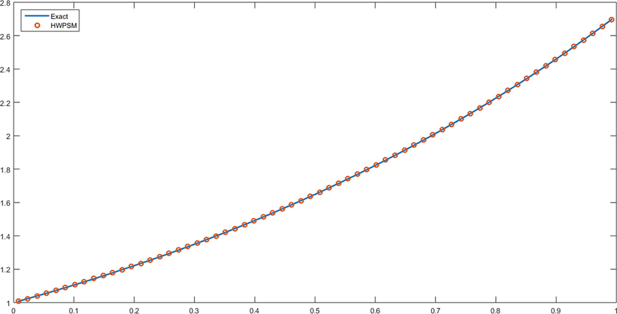
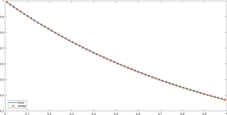
- Graph of problem 1 for J = 5.
| Exact | HWM | Error | |
|---|---|---|---|
| 1 | 0.0625 | 0.0629 | 4.0000E−003 |
| 3 | 0.1864 | 0.1886 | 2.200E−003 |
| 5 | 0.3074 | 0.3099 | 2.500E−003 |
| 7 | 0.4237 | 0.4243 | 6.000E−003 |
| 9 | 0.5333 | 0.5325 | 8.000E−003 |
| 11 | 0.6346 | 0.6386 | 6.000E−003 |
| 13 | 0.7260 | 0.7112 | 1.480E−002 |
| 15 | 0.8061 | 0.8830 | 2.310E−002 |
| Level of Resolution J | Max. abs. Error |
|---|---|
| 3 | 1.5000 E−003 |
| 4 | 8.2354 E−004 |
| 5 | 3.8198 E−004 |
| 6 | 2.0353 E−004 |
| 7 | 1.0458 E−004 |
| 8 | 5.3230E−005 |
| 9 | 2.6683E−005 |
| 10 | 1.3362E−006 |
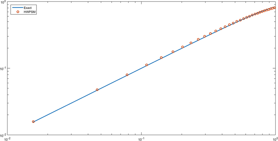
- loglog plot of problem 2 for J = 4.
| Exact | HWM | Error | |
|---|---|---|---|
| 1 | 0.0625 | 0.0629 | 4.000E−004 |
| 3 | 0.1864 | 0.1886 | 2.200E−003 |
| 5 | 0.3074 | 0.3099 | 2.500E−003 |
| 7 | 0.4237 | 0.4243 | 6.000E−003 |
| 9 | 0.5333 | 0.5325 | 8.000E−003 |
| 11 | 0.6346 | 0.6286 | 6.000E−002 |
| 13 | 0.7260 | 0.7112 | 1.480E−002 |
| 15 | 0.7806 | 0.7830 | 2.310E−003 |
| Level of Resolution J | Max. abs. Error |
|---|---|
| 3 | 9.3374E−004 |
| 4 | 5.0517E−004 |
| 5 | 1.5678E−004 |
| 6 | 6.9632E−005 |
| 7 | 3.7205E−005 |
| 8 | 9.6130E−006 |
| 9 | 6.8820E−006 |
| 10 | 1.9670E−006 |
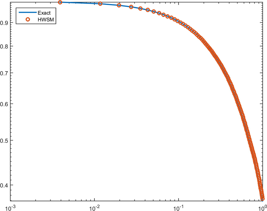
- loglog plot of problem 3 for J = 6.
| Our Method | Wang et al. (2009a) | Wang et al. (2009b) | Wang and Chen (2010) | Lv and Gao (2012) |
|---|---|---|---|---|
| 3.6461E−004 | 2.31E−003 | 5.47E−002 | 5.96E−003 | 9.45E−004 |
| Level of Resolution J | Max. abs. Error |
|---|---|
| 4 | 7.0605E−005 |
| 5 | 1.4873E−005 |
| 6 | 3.6656E−006 |
| 7 | 8.7681E−007 |
| 8 | 2.1541E−007 |
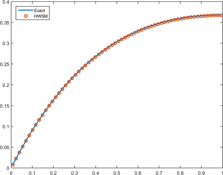
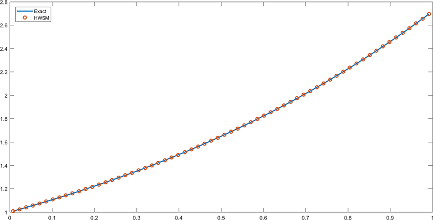
- Plot of problem 4 for J = 5.
| Our Method | Wang et al. (2009a) | Wang et al. (2009b) | Wang and Chen (2010) | Lv and Gao (2012) |
|---|---|---|---|---|
| 8.9532E−005 | 1.85E−003 | 7.66E−002 | 4.94E−003 | 4.01E−004 |
| Level of Resolution J | Max. abs. Error |
|---|---|
| 4 | 1.3456E−005 |
| 5 | 1.9630E−006 |
| 6 | 2.8093E−007 |
| 7 | 3.9528E−008 |
| 8 | 5.4910E−009 |
- Plot of problem 5 for J = 5.
| Exact | HWSM | Error | |
|---|---|---|---|
| 1 | 1.0645 | 1.0608 | 3.700E−003 |
| 3 | 1.2062 | 1.2006 | 5.700E−003 |
| 5 | 1.3668 | 1.3664 | 4.000E−004 |
| 7 | 1.5488 | 1.5463 | 2.500E−003 |
| 9 | 1.7551 | 1.7468 | 8.300E−003 |
| 11 | 1.9887 | 1.9819 | 6.900E−003 |
| 13 | 2.2535 | 2.2485 | 5.000E−003 |
| 15 | 2.5536 | 2.5488 | 4.800E−003 |
| Level of Resolution J | Max. abs. Error |
|---|---|
| 2 | 8.300E−003 |
| 3 | 2.5862E−04 |
| 4 | 4.5075E−05 |
| 5 | 1.3195E−05 |
| 6 | 1.9151E−06 |
- Graph of problem 6 for J = 5.
5 Conclusion
Haar wavelet series method has been applied successfully to solve the linear and nonlinear neutral delay differential equations, which is easy to apply directly. As we have observed that this method has less calculation and takes less time to solve the problems and yield accurate results on increasing the resolution level.
Acknowledgements
We would like to express our sincere gratitude to Professor Khalil Ahmad and the anonymous reviewers for their helpful and valuable comments which greatly improved the quality of the paper.
References
- Adaptive integration of delay differential equations. In: Advances in time-delay systems. Lect. Notes Comput. Sci. Eng.. Vol 38. Berlin: Springer; 2004. p. :155-165.
- [Google Scholar]
- Haar wavelet method for solving lumped and distributed-parameter system. IEEE Proc.-Control Theory Appl.. 1997;144:87-94.
- [Google Scholar]
- An Introduction to Wavelets. San Diego: Academic Press; 1992. p. :49-74.
- Wavelet Transform and Their Application. Springer New york: Birkhauser; 2015. p. :337-440.
- Ordinary and delay differential equations. In: Applied Mathematical Sciences. Vol 20. New York-Heidelberg: Springer-Verlag; 1977. p. :225-331.
- [Google Scholar]
- Introduction to the theory and applications of differential equations with deviating arguments. In: Mathematics in Science and Engineering. Vol 105. New York-London: Academic Press [A Subsidiary of Harcourt Brace Jovanovich, Publishers]; 1973. p. :165-182.
- [Google Scholar]
- Stability and oscillations in delay differential equations of population dynamics. In: Mathematics and its Applications. Vol 74. Dordrecht: Kluwer Academic Publishers Group; 1992. p. :394-461.
- [Google Scholar]
- The Haar wavelets operational matrix of integration. Int. J. Syst. Sci. 1996:623-628.
- [Google Scholar]
- Differential Equations: Stability, Oscillations, Time Lags. New York-London: Academic Press; 1966. p. :394-510.
- The numerical solution of second order boundary value problems by collocation method with Haar wavelets. Math. Comput. Model.. 2010;50:1577-1590.
- [Google Scholar]
- A computational algorithm for large-scale nonlinear time delays systems. IEEE Trans. Syst. Man. Cybern.. 1984;SMC-14:2-9.
- [Google Scholar]
- On the numerical solution of neutral delay differential equations using multiquadric approximation scheme. Bull. Korean Math. Soc.. 2008;45:663-670.
- [Google Scholar]
- Applied theory of functional-differential equations. In: Mathematics and its Applications (Soviet Series). Vol 85. Dordrecht: Kluwer Academic Publishers Group; 1992. p. :48-54.
- [Google Scholar]
- Delay differential equations with applications in population dynamics. In: Mathematics in Science and Engineering. Vol 191. Boston, MA: Academic Press Inc.; 1993. p. :3-116.
- [Google Scholar]
- The waveform relaxation method for time domain analysis of large scale integrated circuits. IEEE Trans. CAD. 1982;1(3):131-145.
- [Google Scholar]
- Application of the Haar wavelet transform to solving integral and differential equations. Proc. Estonian Acad. Sci. Phys. Math.. 2007;56:28-46.
- [Google Scholar]
- The RKHSM for solving neutral functional-differential equations with proportional delays. Math. Methods Appl. Sci. 2012
- [CrossRef] [Google Scholar]
- A computational method based on Hermite wavelets for two-dimensional Sobolev and regularized long wave equations in fluids. Numer. Methods Partial Diff. 2017 Eq.;00:1-23
- [Google Scholar]
- A numerical procedure based on Hermite wavelets for two-dimensional hyperbolic telegraph equation. Eng. Comput. 2017
- [CrossRef] [Google Scholar]
- A haar wavelet approximation for two-dimensional time fractional reaction-subdiffusion equation. Eng. Comput. 2018
- [CrossRef] [Google Scholar]
- Wavelet transform and wavelet-based numerical methods: an introduction. Int. J. Nonlinear Sci.. 2012;13:325-345.
- [Google Scholar]
- Haar wavelet approach for numerical solution of two parameters singularly perturbed boundary value problems. Appl. Math. Inf. Sci.. 2014;8(6):2965-2974.
- [Google Scholar]
- The variational iteration method for solving a neutral functional-differential equation with proportional delays. Comput. Math. Appl.. 2010;59:2696-2702.
- [Google Scholar]
- Stability of continuous Runge–Kutta-type methods for nonlinear neutral delay-differential equations. Appl. Math. Model.. 2009;33(8):3319-3329.
- [Google Scholar]
- Stability of one-leg Θ-methods for nonlinear neutral differential equations with proportional delay. Appl. Math. Comput.. 2009;213(1):177-183.
- [Google Scholar]
- Wavelets Made Easy, 978-1-4612-0573-9. Springer; 1999.


