Geometric morphometric discrimination between seven populations of Kawakawa Euthynnus affinis (Cantor, 1849) from Peninsular Malaysia

1 Introduction

Worldwide, there are more than 30,000 fish species, representing more than half of all vertebrates (Wang et al., 2018; Marchetti et al., 2020). Approximately 20,000 marine species; whereby15,000 species and 705 species occurred in both marine and freshwater systems (Vinod et al., 2020). Fish has direct economic value and are valuable animal protein sources for humans, apart from being a significant component of biodiversity (Marchetti et al., 2020). One of the most important species is Kawakawa, E. affinis (Cantor, 1849), which belongs to the Scombridae family and is found throughout the tropical and subtropical waters of Indo‐Pacific regions (Yazawa et al., 2019; Khoa et al., 2021). It is a small epipelagic, migratory, neritic tuna that has become one of Malaysia’s most important commercial tuna species (Masazurah et al., 2012; Yazawa et al., 2015).

Species identification and population discrimination are critical in conserving and managing fisheries resources (Karakulak et al., 2016). Due to its effectiveness in the collection, retention, and visualization of shape details, the geometric morphometric method has been widely used for morphological studies in recent years (Klingenberg, 2015; Watanabe, 2018). The geometric morphometric has the power to distinguish between closely related species of fish (Imtiaz and Md Naim, 2018), and the correlation between shape as well as a difference of developmental, evolutionary, functional, and ecological factors (Polly et al., 2016). The shape and size of the body in geometric morphometrics are key methods for the registry of morphological differences, particularly variations in shape and size (Imtiaz and Md Naim, 2018).

Previous reports conducted on E. affinis was focused mainly on the population dynamics, biological characteristics, reproductive, mortality, and stock assessment (Rohit et al., 2012; Johnson and Tamatamah, 2013; Sulistyaningsih et al., 2014; Nissar et al., 2015; Ardelia et al., 2016; Kumar et al., 2019). In Australian waters, Griffiths et al. (2017) investigated the relationships of morphometric (fork length–total length and length-weight) among four Scombridae fish species (E. affinis, Thunnus tonggol, Rastrelliger kanagurta, and Cybiosarda elegans). To our knowledge, there is no previous study conducted on E. affinis using geometric morphometric techniques in Peninsular Malaysia. Hence, the current research aimed to discriminate the Euthynnus affinis through shape and body size variations and to evaluate the variations among seven populations of E. affinis from the west and east coast of Peninsular Malaysia.

2 Materials and methods

2.1

2.1 Sampling and study area

A total of 114 samples of Euthynnus affinis (Kawakawa) from Peninsular Malaysia were collected from fish landing sites (Table 1, Fig. 1). Samples were collected from two main geographic areas, Straits of Malacca (M) and the South China Sea (SCS). Samples were morphologically identified and confirmed according to Collette and Nauen (1983). Samples were transported to the Molecular Ecology Laboratory, School of Biological Science, Universiti Sains Malaysia and washed with running water upon arrival at the laboratory, tapped, and placed with the left side on a flat surface with a black background for typical visibility. To capture the proper insertion and origin of fins, all fins were erected using pins. All samples were photographed, labeled, and digitized with a digital camera (Nikon, D90). Purified images were used for geometric morphometric analysis. A digital caliper was used to measure morphometric traits (Fig. 2).

Table 1 Sampling size (N) and description of sampling locations.

No	Sampling locations	Coordinates	Marine region	N
1.	Pasir puteh, Kelantan	5° 49′ 58.28″N; 102° 24′ 19.02″E	SCS	18
2.	Tok Bali, Kelantan	5°52′35.5″N; 102027′29.9″E	SCS	14
3.	Pantai Kijal, Terengganu	4°18′20.2″N; 103°28′57.2″E	SCS	8
4.	Pulau Tenggol, Terengganu	4° 47′ 59.99″ N; 103° 40′ 59.99″ E	SCS	21
5.	Sungai Besar, Selangor	3°39′50.4″N; 100059′16.6″E	M	14
6.	Kuala Selangor, Selangor	3° 21′ 0.00″ N; 101° 15′ 0.00″ E	M	24
7.	Kukup, Johor	1° 18′ 60.00″ N; 103° 26′ 59.99″ E	M	15
Total	114	114

Note: South China Sea (SCS), Straits of Malacca (M).

Close

Fig. 1

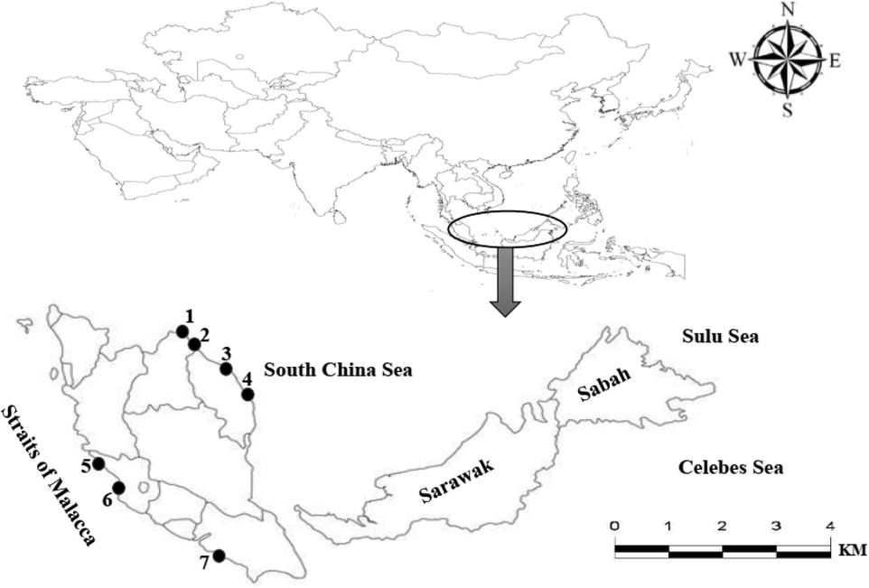
Sampling locations of Euthynnus affinis specimens collected from the Straits of Malacca and South China Sea: 1. Pasir Puteh, Kelantan, 2. Tok Bali, Kelantan, 3. Pantai Kijal, Terengganu, 4. Pulau Tenggol, Terengganu, 5. Sungai Besar, Selangor, 6. Kuala Selangor, Selangor, 7. Kukup, Johor.

Export to PPT

Close

Fig. 2

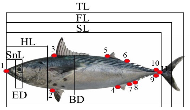
Locations of 11 landmarks and description of 20 variables with seven morphometric measurements of Euthynnus affinis (Kawakawa). TL: total length, FL: fork length, SL: standard length, HL: head length, BD: body depth, ED: eye diameter, SnL: snout length. 1--3: tip of the snout to the first dorsal fin, 3--2: first dorsal fin to pelvic fin, 1--2: tip of the snout to pelvic fin, 3--5: first dorsal fin to second dorsal fin, 5--4: second dorsal fin to the origin of anal fin, 5--7: second dorsal fin to insertion of anal fin, 2--4: pelvic fin to the origin of anal fin, 5--6: second dorsal fin to first superior finlets, 6--8: first superior finlets to first inferior finlets, 4--8: origin of the anal fin to first inferior finlets, 6--10: first superior finlets to the last superior finlets, 10--9: last superior finlets to the last inferior finlets, 8--9: first inferior finlets to the last inferior finlets, 3--4: first dorsal fin to the origin of anal fin, 2--5: pelvic fin to second dorsal fins, 5--8: second dorsal fin to first inferior finlets, 4--6: origin of the anal fin to first superior finlets, 6--9: first superior finlets to last inferior finlets, 8--10: first inferior finlets to last superior finlets, 1--11: standard length.

Export to PPT

3 Results

3.2

3.2 Shape differences of body size in Euthynnus affinis

A total of 20 variables were constructed from 11 homologous landmarks and used to differentiate the taxa based on body shape differences within E. affinis species (Fig. 2).

The PCA analysis of 114 data revealed 18 components that were used to determine body shape and size differences. With a variance of 24.35 percent, the first component had an eigenvalue of 0.017 percent, indicating low significance [an eigenvalue larger than 0.3 is deemed significant (Lombarte et al., 2012)]. Nevertheless, the first four PCs explained 24.35% (PC1: body depth, head, dorsal fin, anal fin, caudal fin, and body size), 19.09% (PC2: body depth, head, dorsal fin, anal fin, and body size), 11.29% (PC3: body depth, anal fin, caudal fin, and body size), and 10.96% (PC4: body depth, head, dorsal fin, anal fin, caudal fin, and body size), respectively with a common variance of 65.69% to demonstrate body shape differences in 2 dimensions (Figs. 3, 4 and 6).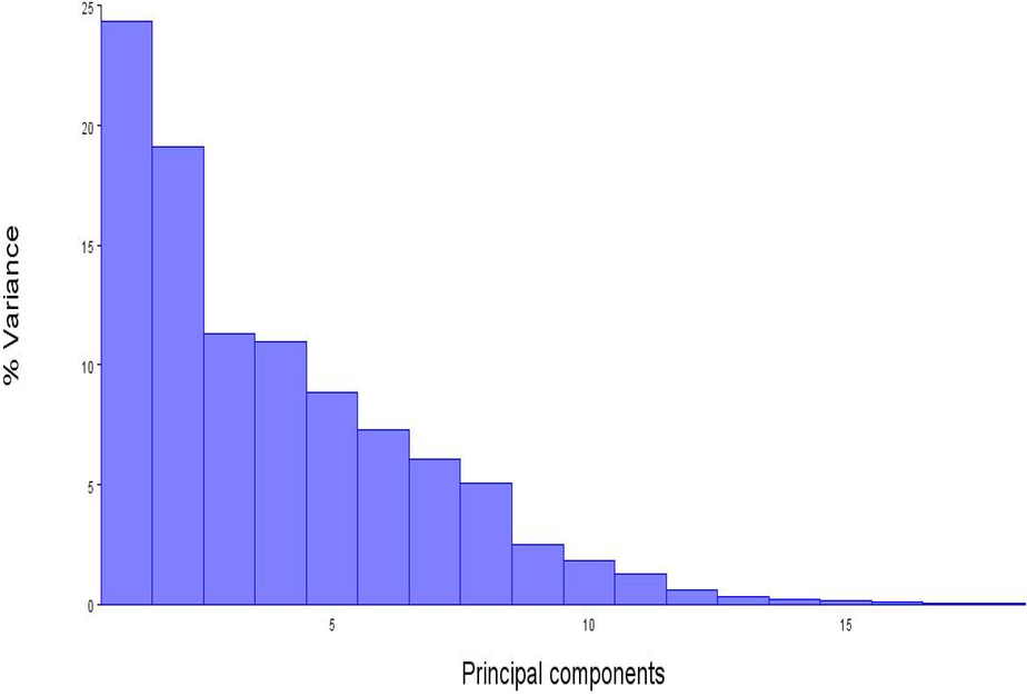

Close

Fig. 3

Values of all principal components plotted against total variation (%) among (114 individuals) of Euthynnus affinis.

Export to PPT

Close

Fig. 4

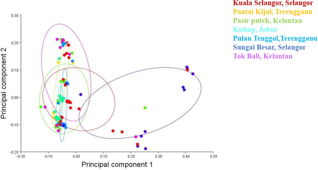
Principal components analysis of seven population of Euthynnus affinis shows PC1 = 24.35%, PC2 = 19.09%, PC3 = 11.29, and PC4 = 10.96, accounting for 65.69% of the total variation in 114 samples.

Export to PPT

The overlapping patterns in the scatterplot of PC1 versus PC2 (Fig. 4) confirmed the limited differences in body shapes of E. affinis, with a very low eigenvalue (less than 0.3) that was not significant to distinguish individuals identified as E. affinis based on the common body shape. A cluster analysis (UPGMA) based on the procrustes distances revealed that the average shapes of populations from Terengganu, Kelantan, and Johor were morphological homogenous. In contrast, the average shapes of populations from Selangor were separated (Fig. 5). To put it another way, Figs. 4 and 5 showed that the populations were mixed up with no evident of division, implying that physical homogeneity existed between the populations from Peninsular Malaysia's east coast (Terengganu, Kelantan, and Johor). The populations of Peninsular Malaysia's west coast (Selangor) were segregated and formed a different group/cluster.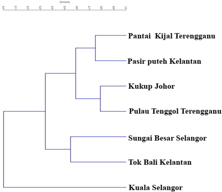

Close

Fig. 5

Dendrogram generated by Unweighted Pair Group Method with Arithmetic Mean (UPGMA) algorithm using procrustes distances between seven populations of Euthynnus affinis collected from Peninsular Malaysia.

Export to PPT

Close

Fig. 6

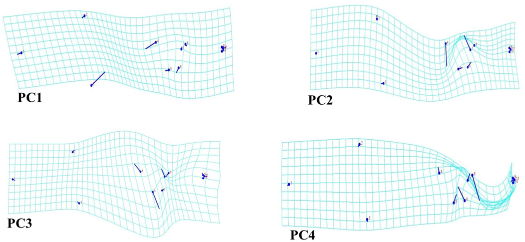
Visualization of shape variations between PC1 to PC4 by wireframe explaining shape variations. PC1 shows changes in body depth, head, dorsal fin, anal fin, caudal fin, body size. PC2 shows changes in body depth, head, dorsal fin, anal fin, caudal fin, body size. PC3 shows the changes in body depth, anal fin, caudal fin, body size. PC4 shows changes in body depth, head, dorsal fin, anal fin, caudal fin, body size.

Export to PPT

Seven morphometric variables in the E. affinis population were studied using DFA analysis. Six functions were identified in the DFA analysis, namely functions 1, 2, 3, 4, 5, and 6, with variances of 74.1%, 19.9%, 3.8%, 1.1%, 0.9%, and 0.3%, respectively. Therefore, the first three functions showed a significant correlation for population discrimination with the value of 0.97, 0.89, and 0.66, respectively (Table 2). For testing function 1 through function 6 (Wilk's lambda = 0.005), function 2 through function 6 (Wilk's lambda = 0.077), function 3 through function 6 (Wilk's Lambda = 0.38), and function 4 through function 6 (Wilk's lambda = 0.67), the Wilk's lambda statistic had a probability of p = 0.000 (Table 2). It is regarded that body depth (B.D) (0.83) scores the highest followed by standard length (SL) (0.78), fork length (F.L) (0.77), total length (T.L) (0.75), eye diameter (E.D) (0.57), and head length (H.L) (0.55) when placing into DFA analysis based on the scoring of variables in function 1. In contrast, snout length (SnL) (0.67) scores the highest in functions 4 (Table 3). Thus, based on the DFA analysis, the prediction group membership between seven populations of Euthynnus affinis are Pasir Puteh (PP) and Tok Bali (TB) (Kelantan), Pantai Kijal (PK) and Pulau Tenggol (PT) (Terengganu), Sungai Besar (SB) and Kuala Selangor (KS) (Selangor), and Kukup (Ku) (Johor) (Table 4).

Table 2 Eigenvalue and Wilk’s lambda of each function of DFA of Euthynnus affinis from Peninsular Malaysia. (a) indicates the first six discriminant functions used in the analysis.

Function	Eigenvalue	% Of variance	Cumulative %	Canonical correlation	Wilks' Lambda	Sig.
1	14.780a	74.1	74.1	0.968	0.005	0.000
2	3.971a	19.9	94.0	0.894	0.077	0.000
3	.755a	3.8	97.8	0.656	0.382	0.000
4	.211a	1.1	98.9	0.417	0.670	0.000
5	.172a	0.9	99.7	0.384	0.812	0.001
6	.051a	0.3	100.0	0.220	0.952	0.072

Table 3 Structure matrix of distributed correlation among measurement characteristics with functions for morphometric characteristics.

Variables	Function
	1	2	3	4	5	6
B.D	0.832*	−0.382	0.363	−0.006	−0.111	−0.019
S.L	0.784*	0.420	−0.167	0.197	−0.319	0.034
F.L	0.774*	0.406	−0.044	0.291	−0.218	−0.085
T.L	0.747*	0.288	−0.030	0.399	−0.419	−0.154
E.D	0.567*	0.539	−0.142	0.098	0.469	0.008
H.L	0.552*	0.374	0.523	0.330	−0.214	0.336
Sn.L	0.374	−0.376	−0.008	0.673*	−0.098	0.485

* Largest absolute correlation between each variable and any discriminant function.

Table 4 Correct classification for seven populations of Euthynnus affinis (88.6%) into their original populations collected from west and east coast of Peninsular Malaysia.

Classification Results
Predicted Group Membership
Original count	State	PP-Kelantan	TB-Kelantan	PK-Terengganu	PT-Terengganu	SB-Selangor	KS-Selangor	PKu-Johor	Total
	PP-Kelantan	14	1	0	0	3	0	0	18
	TB-Kelantan	0	9	0	0	4	1	0	14
	PK-Terengganu	1	0	7	0	0	0	0	8
	PT-Terengganu	0	0	0	21	0	0	0	21
	SB-Selangor	1	2	0	0	11	0	0	14
	KS-Selangor	0	0	0	0	0	24	0	24
	Ku-Johor	0	0	0	0	0	0	15	15
%	PP-Kelantan	77.8	5.6	.0	.0	16.7	.0	.0	100.0
	TB-Kelantan	.0	64.3	.0	.0	28.6	7.1	.0	100.0
	PK-Terengganu	12.5	.0	87.5	.0	.0	.0	.0	100.0
	PT-Terengganu	.0	.0	.0	100.0	.0	.0	.0	100.0
	SB-Selangor	7.1	14.3	.0	.0	78.6	.0	.0	100.0
	KS-Selangor	.0	.0	.0	.0	.0	100.0	.0	100.0
	Ku-Johor	.0	.0	.0	.0	.0	.0	100.0	100.0

4 Discussion

Body shape and size is the main tool for documenting, in particular morphological variations, variations in shape and size, and for assessing taxa relationships based on changes in body shape, even among closely related species of fish (Imtiaz and Md Naim, 2018). The biological shape is quantified by geometrical morphometric variables that preserve geometric configurations of landmarks (Adams et al., 2011).

The results of this study showed that morphological homogeneity existed between communities from Peninsular Malaysia's east coast (Terengganu, Kelantan, and Johor). However, the population of Peninsular Malaysia's west coast (Selangor) was separated from the population of Peninsular Malaysia's east coast, forming a new group/cluster (Fig. 4). These PCA results were further confirmed by the UPGMA created on the Procrustes distances (Fig. 5). Morphological homogeneity based on body shape variations was also reported in the threadfin bream, Nemipterus mesoprion by Joseph and Jayasankar (2001). Generally, our findings are similar to Sajina et al. (2011) which demonstrated that the shape variations of the populations of Megalaspis cordyla (horse mackerel) in the Bay of Bengal and the Arabian Sea were distinct. Similarly, Moreira et al. (2020) found that the blue jack mackerel (Trachurus picturatus) populations in the North Atlantic were separated. Geographical separation may cause the formation of distinct morphological features across fish populations, most likely as a result of the interaction of genetics, environment, and selection that generates morphometric differences within a species (Sajina et al., 2011). Specifically, the Malay Peninsula has been confirmed to be a common land barrier in different species, including fishes in which their dispersal depends on sea currents (Adibah et al., 2015).

In this current study, the first four PCs addressed more than 50% of body shape (particularly body depth, head, dorsal fin, anal fin, caudal fin, and body size) changes in an overall dataset (Figs. 3, 4 and 6). These findings are congruent with the results reported by Claverie et al. (2014) that the first four PCs resulted in 75.3% of shape differences in the reef fishes. The same results were also demonstrated in studies by Geiger et al. (2016) (81.3% of body shape differences in the hybrid complex of Barbus spp.) and Karakulak et al. (2016) (71.3% of body shape differences in Thunnus thynnus and Euthynnus alletteratus). Likewise, Imtiaz and Md Naim (2018) divulged that the first four PCs recovered 80% of shape differences in the Genus Nemipterus. Specifically, we found that the changes in the body shape of E. affinis occurred in the body depth and the overall body shape. Thus, these findings are similar to Bilici et al. (2015) who discovered that morphological variations among Cyprinion macrostomus (Cyprinidae) are based on the variations of the head region and body size of the fish. The geometric morphometrics study conducted by Imtiaz and Md Naim (2018) on the Genus Nemipterus was also discovered the important role of body shape in discrimination between the genus. Similarly, Moreira et al. (2020) found that distances associated with body width and caudal peduncle were the most important variables explaining variation across blue jack mackerel (Trachurus picturatus) populations from the North Atlantic. In general, many factors play an important role in morphological variations, for instance, environmental factors, genetic factors, habitat diversity (Bilici et al., 2015), abiotic and biotic components for example food availability, salinity, radiation, temperature, current flow, and water depth (Mustikasari et al., 2020). Additionally, the marine ecosystem which has several different zones of ecological characters, such as penetration of sunlight, availability of food, and speed of the water was also identified as a factor for such changes (Imtiaz and Md Naim, 2018).

Fish, more than any other vertebrates, show more variations in morphological features both within and between populations, and are more sensitive to these changes, eventually changing their morphology (Verma et al., 2014). Morphometric differences across stocks are predicted due to the geographical split between stocks and the origin of distinct ancestors. It is difficult to understand why there are morphological variations between populations, however, it was proposed that genetic, environmental, and interaction between them have determined the morphological characteristics (Aminan et al., 2020).

With a variance of 74.1% and Wilk's lambda scores of 0.000, function 1 contributed the most to identifying E. affinis in DFA analysis of morphometric data (Table 2). Body depth (BD) is shown to play a substantial role in identifying E. affinis with the highest contribution score when loading into the analyses (Table 3), followed by standard length (SL), fork length (FL), total length (TL), eye diameter (ED), and head length (HL) in function 1. Our findings further support the report by Verma et al. (2014) and Darlina et al. (2011) who showed that the first and second functions (function 1 and function 2) in the DFA analysis were able to separate between populations of Clupisoma garua and Rastrelliger spp., respectively. Variations in morphometric characteristics were due to external factors such as water quality and food availability (Sawalman and Madduppa, 2020) as well as dependent and independent factors (Kumar et al., 2019). Additionally, differences in the head of pattern morphology are also due to the use of various environmental niches, availability of food, and type of prey (Darlina et al., 2011; Cronin-Fine et al., 2013).

The DFA analysis was completed by the prediction group membership of E. affinis. The high degree of similarity of the components evaluated in the analysis (Aminan et al., 2020) was used to predict group membership data. DFA studies revealed considerable variations across the seven E. affinis populations in general. Moreira et al. (2020) found a high proportion (88.6%) of the total correctly classified for all seven populations (Table 3) for blue jack mackerel (Trachurus picturatus) from six locations in the North-East Atlantic (83%). It is suggested that both environmental and genetic differences may have been the cause of the disparity between populations (see Verma et al., 2014).

5 Conclusion

The present study is the first attempt at a geometric morphometric approach conducted on the E. affinis from Peninsular Malaysia waters. Principal component analysis and discriminant function analysis successfully revealed the significant variations among body shape between the seven populations of E. affinis examined. Further studies need to combine morphometric and molecular approaches to get accurate discrimination among E. affinis populations.

References

- Morphometrics and phylogenetics: Principal components of shape from cranial modules are neither appropriate nor effective cladistic characters. J. Hum. Evol.. 2011;60(2):240-243.
- [CrossRef] [Google Scholar]
- The Malay Peninsula as a barrier to gene flow in an Asian horseshoe crab species, Carcinoscorpius rotundicauda Latreille. Biochem. Syst. Ecol.. 2015;60:204-210.
- Morphometric Analysis and Genetic Relationship of Rasbora spp. in Sarawak, Malaysia. TLSR. 2020;31(2):33-49.
- [Google Scholar]
- Reproduction Biology Eastern Little Tuna Euthynnus affinis in the Sunda strait. Jurnal Ilmu Dan Teknologi Kelautan Tropis. 2016;8(2):689.
- Morphological differences among the Cyprinion macrostomus (Cyprinidae) populations in the Tigris River. J. Survey Fisheries Sci.. 2015;2(1):57-67.
- A morphospace for reef fishes: Elongation is the dominant axis of body shape evolution. PLoS ONE. 2014;9(11):e112732.
- Collette, B.B., Nauen, C.E., 1983. FAO Species Catalogue Vol. 2 Scombrids of the world an annotated and illustrated catalog of Tunas, Mackerels, Bonitos, and related species know to date. In FAO Fisheries Synopsis (Vol. 2). FAO Fish. Synop. 125(2).
- Application of Morphometric Analysis to Identify Alewife Stock Structure in the Gulf of Maine. Marine Coastal Fisheries. 2013;5(1):11-20.
- Morphometric and molecular analysis of mackerel (Rastrelliger spp) from the west coast of Peninsular Malaysia. Genet. Mol. Res.. 2011;10(3):2078-2092.
- Combining geometric morphometrics with molecular genetics to investigate a putative hybrid complex: A case study with barbels Barbus spp. (Teleostei: Cyprinidae) J. Fish Biol.. 2016;88(3):1038-1055.
- Morphometric relationships for four Scombridae fish species in Australian waters. J. Appl. Ichthyol.. 2017;33(3):583-585.
- Hammer, Ø., Harper, D.A., Ryan, P.D., 2001. PAST: Paleontological statistics software package for education and data analysis. Paleontol. Electron. 4, 3–9.
- Geometric morphometrics species discrimination within the genus nemipterus from Malaysia and its surrounding seas. Biodiversitas. 2018;19(6):2316-2322.
- Length frequency distribution, mortality rate, and reproductive biology of Kawakawa (Euthynnus affinis-cantor, 1849) in the coastal waters of Tanzania. Pak. J. Biol. Sci.. 2013;16(21):1270-1278.
- Morphometric and genetic variations in the threadfin bream Nemipterus mesoprion. J. Mar. Biol. Ass. India. 2001;43(1&2):217-221.
- Morphometric differentiation between two juvenile tuna species [Thunnus thynnus (Linnaeus, 1758) and Euthynnus alletteratus (Rafinesque, 1810)] from the Eastern Mediterranean Sea. J. Appl. Ichthyol.. 2016;32(3):516-522.
- Changes in early digestive tract morphology, enzyme expression and activity of Kawakawa tuna (Euthynnus affinis) Aquaculture. 2021;530:735935.
- MorphoJ: An integrated software package for geometric morphometrics. Mol. Ecol. Resour.. 2011;11(2):353-357.
- Analyzing fluctuating asymmetry with geometric morphometrics: Concepts, methods, and applications. Symmetry. 2015;7(2):843-934.
- Fishery and length based population parameters of little tuna, Euthynnus affinis (Cantor, 1849) from Gulf of Mannar, Southwestern Bay of Bengal. Indian J. Geo Mar. Sci.. 2019;48:1708-1714.
- Ecomorphological analysis as a complementary tool to detect changes in fish communities following major perturbations in two South African estuarine systems. Environ. Biol. Fishes. 2012;94(4):601-614.
- Determining the Authenticity of Shark Meat Products by DNA Sequencing. Foods. 2020;9(9):1194.
- Masazurah, A.R., N, S. A. M., Samsudin, B., 2012. A preliminary study of population structure of kawakawa, Euthynnus affinis (Cantor 1849) in the straits of Malacca. IOTC-2012-WPNT02-23, (Cantor 1849), 1–10.
- Landmark-based geometric morphometrics analysis of body shape variation among populations of the blue jack mackerel, Trachurus picturatus, from the North-East Atlantic. J. Sea Res.. 2020;163:101926.
- Morphological Variation of Blue Panchax (Aplocheilus panchax) Lives in Different Habitat Assessed Using Truss Morphometric. J. Biol. Biol. Educ.. 2020;12(3):399-407.
- Reproductive biology of little tuna (Euthynnus affinis) in the Arabian sea. Ecol. Environ. Constr.. 2015;21(4):115-118.
- Combining geometric morphometrics and finite element analysis with evolutionary modeling: towards a synthesis. J. Vertebr. Paleontol.. 2016;36(4):e1111225.
- Fishery and bionomics of the little tuna, Euthynnus affinis (Cantor, 1849) exploited from Indian waters. Indian J. Fisheries. 2012;59(3):33-42.
- Stock structure analysis of Megalaspis cordyla (Linnaeus, 1758) along the Indian coast based on truss network analysis. Fish. Res.. 2011;108(1):100-105.
- The Analysis of Morphological and Genetic Characteristics of Yellowstripe Scad from Muara Baru Modern Fish Market in North Jakarta. Jurnal Ilmiah Perikanan Dan Kelautan. 2020;12(2):308-314.
- Sulistyaningsih, R.K., Jatmiko, I., Wujdi, A., 2014. Length Frequency Distribution and Population Parameters of Kawakawa (Euthynnus affinis-Cantor, 1849) Caught by Purse Seine in the Indian Ocean (a Case Study in Northwest Sumatera IFMA 572). IOTC–2014–WPNT04–20, 1–14.
- Phylogeny Based on Truss Analysis in Five Populations of Freshwater Catfish: Clupisoma Garua. Int. J. Sci. Res. (IJSR). 2014;3(8):1414-1418. Retrieved from
- DNA barcode profiling and intraspecies variation analysis within the barcode region of an ornamental red lion fish-Pterois volitans (Linnaeus, 1758) J. Interdiscip. Cycle Res.. 2020;12(8):339-357.
- DNA barcoding of marine fish species from Rongcheng Bay, China. PeerJ. 2018;2018(6):1-19.
- How many landmarks are enough to characterize shape and size variation? PLoS ONE. 2018;13(6):1-17.
- GnRHa-induced spawning of the Eastern little tuna (Euthynnus affinis) in a 70–m3 land-based tank. Aquaculture. 2015;442:58-68.
- Production of triploid eastern little tuna, Euthynnus affinis (Cantor, 1849) Aquac. Res.. 2019;50(5):1422-1430.
- Developmental regulation of skull morphology II: Ontogenetic dynamics of covariance. Evol. Dev.. 2004;8(1):46-60.