

Translate this page into:
Fractional partial differential equations and novel double integral transform
⁎Corresponding author.
-
Received: ,
Accepted: ,
This article was originally published by Elsevier and was migrated to Scientific Scholar after the change of Publisher.
Peer review under responsibility of King Saud University.
Abstract
We propose in this study a combined expression mainly based on the double transformation of Laplace and Sumudu (DLST), by developing some results associated with this proposed transformation. We can apply this double transformation to certain functions to achieve interesting results which can be used to solve certain classes of fractional partial differential equations (FPDE). The numerical results show that this double transformation can lead to an exact solution of linear FPDEs. Laplace-Sumudu transform; Laplace transform; Sumudu transform; Fractional partial differential equations.
Keywords
Double Laplace-Sumudu transform
Sumudu transform
Fractional partial differential equations

1 Introduction
The double integral transform is nevertheless a new and renewed study (see for example Alderremy et al., 2020; Alderremy and Elzaki, 2018; Elzaki, 2012; Waleed et al., 2021) where previous work considered definitions, simple theories of PDEs (Weatugala, 1993; Belgacem and Karaballi, 2002; Belgacem and Karaballi, 2006; Belgacem and Karaballi, 2006b). The combination of the integral transform with other computational techniques, such as Differential Transform Method, Homotopy Perturbation Method, Adomian Method and Variational Iteration Method has been the subject of much work (Ahmed et al., 2020; Elbadri et al., 2020; Mohamed and Elzaki, 2020; Alderremy et al., 2020, Chamekh et al., 2019; Chamekh et al., 2021) to solve differential equations. In this article, we will develop some results using the proposed double integral transformation. As this transform is still under study, we will compare the solutions with solutions obtained with standard methods. For non-linear FPDEs the work needs even more effort in the future to adapt this transformation to these types of equations.
Here we propose to study the FPDEs in the form:
Let
real constants and
is the linear differential operator. We consider resolving the following problem:
2 Preliminaries
Definition: 2.1
The DLST of
, denoted by:
and defined as:
Definition: 2.2
The inverse (DLST)
is defined by:
Definition: 2.3The
th order Caputo derivative (
,
) of
is given by:
Definition: 2.4
The Mittag-Leffer functions
,
and
, is,
The single transform (ST) of
and
takes the form:
3 Fundamental properties of (DLST)
Sr. No
1
2
3
4
5
6
7
8
,
is the zero order Bessel function
9
10
11
3.1 Existence condition for the DLST
If is an exponential order a and ; tend to infinity and if it exist a nonnegative real,
Then:
Theorem 3.1.1
If a function on the interval and of exponential order and , then the DLST of well-defined for all and supplied and
Proof.
We find, from the Def. 2.1,
3.2 Basic derivatives properties of the DLST
If,
, then:
Proof
For (16)
Let, thus:
Concerning (16)
Let, then:
It is easy to prove (17), (18), and (19).
Theorem 3.2.1
If
, thus:
Proof
Using Def. 2.1 Putting,
3.3 Convolution Theorem of DLST
3.4 Definition 3.3.1
The double convolution of
and
is given,
Theorem 3.3.1 (Convolution Theorem)
If
and
then:
Proof
Using Def. 2.1
Using Theorem 3.2.1 to find
4 Principle of DLST method
In this part, we exercised DLST to find the solution to the Eq. (1).
First, apply DLST to Eq. (1), we get:
Furthermore, applying single (LT) to the ICs(2) and single (ST) to the BCs(3), we've got,
5 Elucidative examples
Without forgetting the work of Podlubny 1999, who has proposed some analytical solutions for certain linear equations which can be calculated. We treat in this numerical part some physical applications using the DLST method. The objective is to illustrate the method and prove its applicability.
5.1 Fractional advection-diffusion equation
Putting,
, to find,
WithICs and BCs:
5.2 Fractional reaction-diffusion equation
Putting,
and
in Eq. (1), to get,
With, ICs and BCs:
So,(27) gives a solution of (31) as:
5.2.1 Fractional heat (diffusion) equation
If we choose,
in (31), we got,
With, ICs and BCs:
So, (33) yields the solution of (34)
Example 1: Putting
and
in (34), to yield,
5.3 Fractional telegraph equation
Putting
and
, we’ve got,
So, (27) gives the solution of (41) in the form,
Example 2: If we choose,
and
in (41), we get,
5.3.1 Fractional wave equation
If we choose,
in (41), then, we get,
Fractional Klein–Gordon equation
Putting,
and
, to find,
With ICs and BCs:
So, (27) yields the solution of (51),
Example 3: If we choose,
and
in (51), we have got
5.4 Fractional Burger’s equation
Choosing,
, we obtain,
Example 4: If we choose,
and
in (57) to get,
Replacing,
in (59) and simplifying, to obtain,
5.5 Fractional Fokker-Planck equation
Putting,
and
, to get,
Example 5: If we choose,
in (63) then, we find:
Replacing,
in (65) and simplify it, to find:
5.6 Fractional Korteweg-de Vries (KdV) equation
Putting,
and
in (1), to get,
Example 6: If we choose,
and
in (69) we have:
6 Discussions
We are going look in this section the numeric evaluation of obtained results of fractional equations that have proposed to be solve. Moreover, we will discuss the numerical behavior of the solution resulting from a fractional differential equation and compare it with that of the equation with integer derivative.
When δ = 1, the closed form solution of each Example 3, 4, 5 and 6 is simply calculated. We have opted to examine the numerical results for the values of δ = 0.95, 0.85 and 0.75. We have noticed that the solutions obtained for the different fractional values of δ are in coordination with the solution of closed form for α = 1, as shown in Figs. 1–4. It suffices to clearly notice that when α approaches 1, the solution resulting from the fractional equation approaches this exact solution.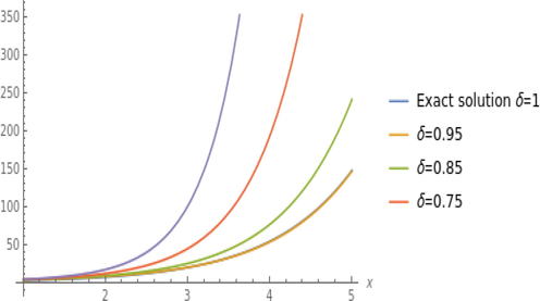
Solutions of Fractional Klein–Gordon.
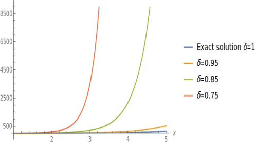
Solutions of Fractional Burger’s.
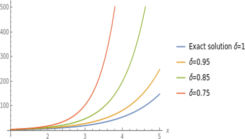
Solutions of Fractional Fokker-Planck.
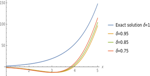
Solutions of Fractional Korteweg-de Vries (KdV).
7 Conclusions
This article deals with the approach of a new double transformation. The objective is based on the simplicity of the technique used to solve a large class of fractional equations of mathematical physics. The examples show that DLST can be a good alternative to treat many LFPDEs that appear in science. However, it should be noted that the solutions obtained are valid while the inverse of this transform exists.
Acknowledgement
This work was funded by the University of Jeddah , Saudi Arabia, under grant No. (UJ-20-101-DR ). The authors, therefore, acknowledge with thanks the University technical and financial support.
Declaration of Competing Interest
The authors declare that they have no known competing financial interests or personal relationships that could have appeared to influence the work reported in this paper.
References
- A new efficient method for solving two-dimensional nonlinear system of Burger’s differential equation. J. Abstr. Appl. Anal. 2020:1-7.
- [Google Scholar]
- Semi-analytical solution for a system of competition with production a toxin in a chemostat. J. Math. Computer Sci.. 2020;20(02):155-160.
- [Google Scholar]
- Analytical investigations of the Sumudu transform and applications to integral production equations. Math. Probl. Eng. (3):103-118.
- [Google Scholar]
- Sumudu transform fundamental properties investigations and applications. J. Appl. Math. Stochast. Anal. 2006:1-23.
- [Google Scholar]
- Semianalytical solution for some proportional delay differential equations. SN Appl. Sci.. 2019;1:148.
- [Google Scholar]
- Approximate analytical solutions for some obstacle problems. J. King Saud Univ. Sci.. 2021;33(2):101259.
- [Google Scholar]
- A new solution of time-fractional coupled KdV equation by using natural decomposition method. J. Abstr. Appl. Anal. 2020:1-9.
- [Google Scholar]
- Double Laplace variational iteration method for solution of nonlinear convolution partial differential equations. Arch. Sci.. 2012;65(12):588-593.
- [Google Scholar]
- On the new double integral transform for solving singular system of hyperbolic equations. J. Nonlinear Sci. Appl.. 2018;11(10):1207-1214.
- [Google Scholar]
- Sumudu transform fundamental properties investigations and applications. J. Appl. Math. Stochast. Anal.. 2006;2006:1-23.
- [Google Scholar]
- Applications of new integral transform for linear and nonlinear fractional partial differential equations. J. King Saud Univ. Sci.. 2020;32(1):544-549.
- [Google Scholar]
- Podlubny, I., 1999 Fractional Differential Equations, vol. 198 of Mathematics in Science and Engineering, Academic Press, San Diego.
- Sumudu transforms - a new integral transform to solve differential equations and control engineering problems. Math. Eng.. 1993;61:319-329.
- [Google Scholar]
- Modified double conformable laplace transform and singular fractional pseudo-hyperbolic and pseudo-parabolic equations. J. King Saud Univ. Sci.. 2021;33:101378
- [Google Scholar]


