Force analysis of unstable section of electrostatic spinning charged jet

Liang Chen; Liang Zhiyong; Lu Li

doi:10.1016/j.jksus.2019.02.008

View/Download PDF

Buy Reprints

PDF

Translate this page into:

31 (

); 1528-1534

doi:

10.1016/j.jksus.2019.02.008

Force analysis of unstable section of electrostatic spinning charged jet

Liang Chen^{^a}, Liang Zhiyong^{^b,⁎}, Lu Li^{^b}

a College of Mechanical Engineering, University of Birmingham Edgbaston Birmingham B15 2TT, UK

b College of Science, Donghua University, Shanghai 201620, PR China

⁎Corresponding author. zhyliang@dhu.edu.cn (Liang Zhiyong)

Received: 2018-11-6, Accepted: 2019-2-10, Published: 2019-10-01

Disclaimer:
This article was originally published by Elsevier and was migrated to Scientific Scholar after the change of Publisher.

Peer review under responsibility of King Saud University.

Abstract

The basic mechanism of electrostatic spinning is rapid whipping of charged jet. An ideal model was established for the key part of electrostatic spinning mathematical model, which is visco-elastic behavior model of the unstable section of charged jet. Through mechanical analysis of the viscoelastic behavior model and calculation of its governing equations, the physical and dynamic properties of the unstable section of the charged jet in the three-dimension Cartesian coordinate system were obtained. It will have a theoretical effect on the development of electrostatic spinning technology.

Keywords

Electrostatic spinning

Charged jet

Rapid whipping

Viscoelastic behavior model

Mechanical analysis

Show Related Articles from PubMed

1 Introduction

The electro-spinning method is a new spinning method for preparing polymer nanofibers by using electrostatic field force (Jianzong, 2012), which is of great significance for mathematical modeling. In the known literature, the mathematical model of electro-spinning can be divided into two types: the first type of model uses the equation of continuum mechanics to describe the charged jet, which focuses on the microscopic mechanical properties of the charged jet, i.e. hydrodynamics, Based on computational fluid dynamics and visco-elastic mechanics, the motion law of charged jet under external action is studied from a unified point of view. For example, Shin et al. (2001) proposed the electro-hydrodynamic model of Newtonian liquid jet; the second model uses Newtonian mechanics. The equation describes the charged jet, which focuses on the macroscopic mechanical properties of the charged jet, that is, based on Newton's law of motion, the motion law of the charged jet is studied. For example, Yarin and Zussman (2004) proposed a dimensionless bead connected by a damper and a spring model. Therefore based on the different characteristics and the relationship between the two types of mechanical models, a new mechanical model of the unstable segment of the charged jet, the visco-elastic behavior model, can be established.

Considering the macroscopic and microscopic mechanical properties of the charged jet, this paper firstly establishes a new mechanical model of the charged jet unstable section, and analyzes the force, and then establishes the ideal behavior of the charged jet under the three-dimension Cartesian coordinate system, Coupled control equations.

Considering the ideal motion of the unstable segment of the charged jet and the parameter calculation of the mechanical model, the mechanical model of the unstable segment of the charged jet proposed in this paper is based on the following assumptions, see Fig. 1.

Continuous charged jet trajectories and ideal micro element jet models.

1.1

1.1 Hypothesis and establishment of a mechanical model for unstable segments with charged jets

(1)

The electrospinning process starts from the needle (Theron et al., 2005).
(2)

The charged jet process does not consider the case where the main jet splits into a secondary jet (Yarin and Zussman, 2004).
(3)

The fluid unit of the jet is made up of a model of an elongated segment cylinder, which is only subjected to axial forces.
(4)

The polymer solution contains only the embedded charge, and its transport is only carried out by the movement of the fluid unit of the jet (Yarin and Zussman, 2004).
(5)

The viscoelastic behavior of the polymer solution can be described by a nonlinear Maxwell flow model (Yarin and Zussman, 2004).
(6)

The mass transport of the solvent between the charged jet and the surrounding gaseous medium is described by Fick's first law (Theron et al., 2005).
(7)

The external electrostatic field is calculated by vector superposition by the electric field excited by the charge carried by the charged jet (Shin et al., 2001).

1.2

1.2 Mass transport equation of solvent between charged jet and surrounding gaseous medium

The solvent will volatilize during the movement of the charged jet. In order to facilitate the calculation of the governing equation, it is necessary to consider the mass exchange between the charged jet and the surrounding gaseous medium (air).

Fick's first law describes the large amount of solvent transport between the jet in the rotating space and the surrounding medium (Yarin and Zussman, 2004; Theron et al., 2005; Weiya et al., 2014 ), as shown in Eq. (1).

(1)

\frac{d m_{i}}{d t} = h_{m} π d_{i} l_{i} ρ c_{s}^{eq} (1 - RH)

where \{\begin{matrix} \begin{matrix} h_{m} = \frac{0.495 {Re}^{\frac{1}{3}} S_{c}^{\frac{1}{2}} D_{s,a}}{d_{i}} \\ Re = ρ_{a} l_{i} \frac{|v_{i}|}{μ_{a}} \\ S_{c} = \frac{μ_{a}}{ρ_{a} D_{s,a}} \end{matrix} \end{matrix}

where

m_{i},

d_{i},

l_{i}

the instantaneous mass, instantaneous diameter, and instantaneous length of the straight segment of the i-th segment jet micro-element;

h_{m}

is the mass transfer coefficient;

ρ

is the density of the polymer solution;

c_{s}^{eq}

is the concentration of solvent in saturated steam at ambient temperature;

RH

is the relative humidity of the environment;

D_{s,a}

is the binary diffusion coefficient of solvent to air;

Re

is the Reynolds number;

S_{c}

is the Schmitt number. By the calculation, the following formula (2) can be obtained.

(2)

\frac{d m_{i}}{d t} = 0.495 ν_{a}^{\frac{1}{6}} D_{s, a}^{\frac{1}{2}} π ρ c_{s}^{eq} (1 - RH) l_{i}^{\frac{4}{3}} \cdot {|v_{i}|}^{\frac{1}{3}}

where:

μ_{a}

v_{a}

are the dynamic viscosity and kinematic viscosity of air;

v_{i}

is the instantaneous velocity of the straight segment of the jet stream of the i-th segment.

In order to facilitate the next calculation, we define $β_{i}$ as the ratio of the instantaneous volume $V_{i}$ of the straight segment of the jet stream of the i-th segment to the instantaneous volume $V_{0}$ of the straight segment of the initial jet (i.e. the volume scale factor), which is calculated as shown in Eq. (3)

(3)

β_{i} = \frac{V_{i}}{V_{0}} = \frac{l_{i} d_{i}^{2}}{l_{0} d_{0}^{2}}

where:

v_{0}

d_{0}

and

l_{0}

are the initial volume, initial diameter, and initial length of the straight segment of the initial jet micro-element.

1.3

1.3 Visco-elastic behavior model and constitutive equation of charged jet

In order to correctly describe the visco-elastic behavior of the charged jets in unstable sections, we use two different nonlinear rheological models to represent the different stages of jet motion. In the initial stage of the jet motion, because of the high content of solvent in the jet, a new model of the solution in which the solute and the solvent model are connected in parallel is used. The solute model is represented by a series of linear springs and viscous dampers, and the solvent model is represented by another viscous damper. In the final stage of the jet motion, the solvent volatizes with the movement of the jet and the content is less and less, and finally only the solute remains. Therefore, this stage can be used in the nonlinear Maxwell flow model, which can only describe the stress relaxation process of viscoelastic fluids.

1.2.1 When the solvent content in the unstable section jet is high, that is, in the initial stage, the constitutive equation of the described model is as shown in Eqs. (4)–(6). Wherein: formula (4) is a solute model; formula (5) is a solvent model; and formula (6) is a solution model.

(4)

σ_{1} + τ_{1} {\dot{σ}}_{1} = μ_{1} \dot{ε}

(5)

σ_{2} = μ_{2} \dot{ε}

(6)

σ = σ_{1} + σ_{2} = - τ_{1} {\dot{σ}}_{1} + (μ_{1} + μ_{2}) \dot{ε}

For the creep process of a viscoelastic fluid the stress remains constant $σ = σ_{0}$ . Both sides of Eq. (6) simultaneously derive the time t, and the following Eqs. (7) and (8) can be obtained by calculation.

(7)

δ_{1} = C_{1} + C_{2} e^{- \frac{μ_{1} + μ_{2}}{μ_{1} μ_{2}} t}

(8)

δ_{2} = [C_{1} + C_{2} \frac{(τ_{2} - τ_{1}) μ_{1} - τ_{1} μ_{2}}{μ_{1}} e^{- \frac{μ_{1} + μ_{2}}{μ_{1} μ_{2}} t}] \frac{μ_{2}}{μ_{1}}

where:

δ_{0}

is the initial stress to which the viscoelastic fluid is subjected;

δ_{1}

δ_{2}

, and

δ

are the stresses of the solute, solvent, and solution in the viscoelastic fluid, respectively;

τ_{1}

and

τ_{2}

are the relaxation times of the solute and the solvent, respectively;

μ_{1}

μ_{2}

are the kinetic viscosity of the solute and solvent, respectively. When t = 0, the following formula (9) can be obtained from the Eqs. (7) and (8).

(9)

\{\begin{matrix} C_{1} + C_{2} = σ_{1 (0)} \\ C_{1} \frac{μ_{2}}{μ_{1}} + C_{2} \frac{μ_{2}}{μ_{1}} \frac{(τ_{2} - τ_{1}) μ_{1} - τ_{1} μ_{2}}{μ_{1}} = σ_{2 (0)} \end{matrix}

where:

δ_{1} (0) δ_{2} (0)

are the initial stresses of the solute and solvent at t = 0.

In summary, for the straight section of the first-stage jet micro-element, when the solvent content is high, the viscoelastic behavior model is shown in Eq. (10).

(10)

σ_{i} = σ_{1 i} + μ_{2 i} \frac{(r_{i} - r_{i + 1}) \cdot (v_{i} - v_{i + 1})}{l_{i}^{2}}

where:

δ_{i}

and

δ_{1 i}

are the stresses of the solution and solute in the jet fluid of the i-th segment;

μ_{2 i}

is the dynamic viscosity of the solvent in the jet microfluidic fluid;

r_{i}

and

r_{i + 1}

are the instantaneous radius vectors of the straight segments of the jet micro-element of the i-th and (i + 1)th segments respectively;

v_{i}

and

v_{i + 1}

are the instantaneous velocity vectors of the straight segments of the jet micro-element of the i-th segment and the (i + 1)th segment, respectively.

1.2.2 When the content of solvent in the unstable section jet is low, that is, in the final stage, the constitutive equation of the described Maxwell flow model of viscoelastic fluid is shown in Eq. (11).

(11)

\{\begin{matrix} σ + τ \dot{σ} = μ \dot{ε} \\ σ = σ_{0} e^{- \frac{t}{τ}} \\ E = E_{0} e^{- \frac{t}{τ}} \end{matrix}

where:

δ_{0}

is the initial stress of the viscoelastic fluid;

E_{0}

is the initial elastic modulus of the viscoelastic fluid;

τ

is the relaxation time. Therefore, for the straight segment of the

i

-th segment jet micro-element, when the solvent content is low, the viscoelastic behavior model is expressed in Eq. (12).

(12)

\{\begin{matrix} \begin{matrix} \frac{d δ_{i}}{d t} = \frac{μ_{i}}{τ_{i}} \frac{{(r}_{i} - r_{i + 1}) \cdot (v_{i} - v_{i + 1})}{l_{i}^{2}} - \frac{δ_{i}}{τ_{i}} \\ μ_{i} = 10^{{Bw}_{p_{i}}^{m}} \\ B = {log}_{10} \frac{μ_{0}}{w_{p_{0}}^{m}} \\ τ_{i} = \frac{τ_{0}}{w_{p_{0}}} w_{p_{i}} \\ w_{p_{i}} = \frac{m_{p}}{m_{p} + m_{i}} \end{matrix} \end{matrix}

where:

δ_{i}

μ_{i}

τ_{i}

are the instantaneous normal stress, instantaneous dynamic viscosity, and instantaneous relaxation time of the straight segment of the first jet micro-element;

r_{i}

and

r_{i + 1}

are the instantaneous radius vectors of the straight segments of the jet micro-element of the i-th segment and the (i + 1)th segment respectively;

v_{i}

and

v_{i + 1}

are the instantaneous velocity vectors of the jet segments of the i-th segment and the i + 1th segment respectively;

w_{p_{i}}

is the instantaneous polymer mass fraction of the i-segment jet straight segment;

τ_{0}

is the initial relaxation time of the polymer;

w_{p_{0}}

is the initial mass fraction of the polymer solution;

μ_{0}

is the initial kinematic viscosity of the polymer;

m_{p}

is the mass of the polymer;

m

is the index.

1.4

1.4 Calculation of applied electric field strength

The applied electric field is separated from the needle by a certain distance, which not only can stabilize the jet of the straight line segment, but more importantly, it stretches and accelerates the movement of the unstable section of the charged jet, thereby making the electro spun fiber finer.

In this paper, the grounded disc type current collector is used. The electric field between the needle and the grounded disc collector can be considered as a system composed of a charged jet and a current collector composed of infinitesimal cylindrical jet micro-elements (Shin et al., 2001). Assuming that the point where the needle hole is located is the Cartesian coordinate system origin O(x, y, z), see Fig. 2. Each segment of the cylindrical segment of the jet micro-element is uniformly charged, and the grounded disk-type current collector is regarded as an infinite conductive plane. Then the electric field distribution calculation can adopt the “mirror method” model, that is, construct a virtual point charge (mirror charge Q), and the charged symbol of the charge is completely opposite to the jet charge charged symbol. The charge is placed symmetrically on the upper side of the grounded disc-type current collector, the distance from which to the current collector is equal to the distance from the needle to the current collector (Yarin and Zussman, 2004). This method can satisfy the boundary condition of a constant electrostatic potential, so that a point on the surface satisfies the boundary condition. In this mathematical model it is assumed that the charged jet is ejected from point O and is selected as the top end of the straight section of the initial jet micro-element. The calculation of the electrostatic potential at the jet microelement of the i-th segment is as shown in Eq. (13).

(13)

ϕ = \frac{ρ_{q} \cdot d_{0}^{2} l_{0}}{16 ε_{0} ε_{r}} \cdot \frac{1}{|r_{i}|} - \frac{Q}{4 π ε_{0} ε_{r}} \cdot \frac{1}{|r_{i} - r_{Q}|}

where:

ρ_{q}

is the charge density;

Q

is the charge of the image charge,

Q = \frac{π d_{0}^{2} l_{0}}{4} ρ_{q}

;

ε_{0}

is the vacuum permittivity;

ε_{r}

is the relative dielectric constant of the surrounding medium (air);

r_{i}

is the instantaneous radius vector of the straight segment of the i-th segment jet micro-element. That is

r_{i} = (x_{i}, y_{i}, z_{i})

;

r_{Q}

is the radius vector of the virtual charge, i.e

r_{Q} = (0, 0, 2 h)

; h is the distance between the needle and the grounded disc collector;

d_{0}

and

l_{0}

are the initial diameter and initial length of the straight segment of the initial jet micro-element, respectively. At the top point

(0, 0, l_{0})

of the straight line segment of the initial jet micro-element, the boundary condition is set, that is, since the jet charge at the needle is stably distributed, it is assumed that the electrostatic potential of the point O is always

ϕ_{1}

. Then by substituting the boundary condition and the image charge Q into the Eq. (13), the following Eq. (14) can be obtained.

(14)

φ_{1} \equiv φ [(0, 0, l_{0})] = \frac{ρ_{q d_{0}^{2}}}{16 ε_{0} ε_{r}} - \frac{Q}{4 π ε_{0} ε_{r}} \cdot \frac{1}{2 h - l_{0}}

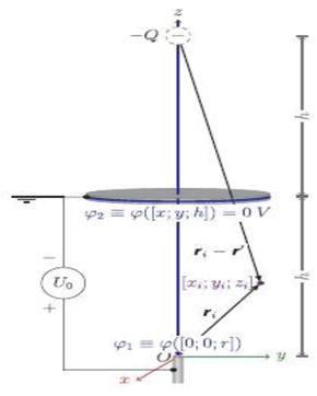
A mathematical and physical model for calculating the distribution of external electric field.

From the formula (14), the following formulas (15) and (16) can be calculated.

(15)

ρ_{q} = \frac{8 ε_{0} ε_{r} ϕ_{1} (2 h - l_{0})}{d_{0}^{2} (h - l_{0})}

(16)

Q = \frac{2 π ε_{0} ε_{r} ϕ_{1} (2 {hl}_{0} - l_{0}^{2})}{h - l_{0}}

By calculating the above parameters, substituting (13) can verify that the electrostatic potential on the plane of the grounded disk collector is zero (because of grounding). According to the above derivation, the electric field strength between the needle and the grounded disk current collector can also be calculated.

Assuming that the electric field intensity generated by the image charge Q at r_i = (x_i, y_i, z_i) is $E_{1}$ , the electric field intensity generated by the stable distributed jet charge at the needle at $r_{i} = (x_{i}, y_{i}, z_{i})$ is $E_{2}$ , then the total field Strong is $E = E_{1} + E_{2}$ . The calculation formula of the electric field strength of the point charge is as shown in Eqs. (17) and (18).

(17)

E_{1} = \frac{- Q}{4 π ε_{0} ε_{r}} \cdot \frac{1}{{|r_{1} - r_{Q}|}^{2}} \cdot \frac{r_{i} - r_{Q}}{|r_{i} - r_{Q}|}

(18)

E_{2} = \{\begin{matrix} \begin{matrix} \frac{ρ_{q}}{3 ε_{0} ε_{rp}} r_{i} & |r_{i}| < l_{0} \\ \frac{ρ_{q} d_{0}^{2}}{16 ε_{0} ε_{r}} \cdot \frac{1}{{|r_{i}|}^{2}} \cdot \frac{r_{i}}{|r_{i}|} & |r_{i}| > l_{0} \end{matrix} \end{matrix}

where:

ε_{rp}

is the relative dielectric constant of the polymer solution. Therefore the total field strength

E

produced by the jet charge at the needle is as shown in Eq. (19).

(19)

E = E_{1} + E_{2} \{\begin{matrix} \begin{matrix} \frac{ρ_{q}}{3 ε_{0} ε_{rp}} r_{i} - \frac{Q}{4 π ε_{0} ε_{r}} \cdot \frac{1}{{|r_{i} - r_{Q}|}^{2}} \cdot \frac{r_{i} - r_{Q}}{|r_{i} - r_{Q}|} & |r_{i}| < l_{0} \\ \frac{ρ_{q} d_{0}^{2}}{16 ε_{0} ε_{r}} \cdot \frac{1}{{|r_{i}|}^{2}} \cdot \frac{r_{i}}{|r_{i}|} - \frac{Q}{4 π ε_{0} ε_{r}} \cdot \frac{1}{{|r_{i} - r_{Q}|}^{2}} \cdot \frac{r_{i} - r_{Q}}{|r_{i} - r_{Q}|} & |r_{i}| > l_{0} \end{matrix} \end{matrix}

Applying a high voltage between the needle and the grounded disk collector creates a strong electrostatic field. Since the distance between the needle and the grounded disk current collector is small, the electric field intensity distribution is relatively uniform, and the direction of the electric field strength can be considered to be approximately vertical to the ground plate. Therefore, the calculation of the electric field strength can adopt the vector superposition rule as shown in the Eq. (20).

(20)

|E| = \sqrt{{|E_{1}|}^{2} + {|E_{2}|}^{2} - 2 |E_{1}| |E_{2}| COS θ}

2 Mechanical analysis of the micro-element of unstable jet volume

After establishing the mechanical model of the unstable section of the charged jet, considering the mass exchange between the charged jet and the external gaseous medium, the behavior of the viscoelastic fluid and the influence of the applied electric field, on this basis, its gravity, applied electric field force, Coulomb force, and viscosity Specific force analysis is performed on elastic force, surface tension and air resistance. Among them, the applied electric field force, Coulomb force, viscoelastic force and surface tension have a crucial influence on the motion of the unstable segment of the charged jet.

2.1

2.1 Gravity

Charged jets are subject to their own weight. Therefore, the gravity of the straight segment of the i-th segment jet micro-element is as shown in Eq. (21).

(21)

G_{i} = m_{i} g = ρ \frac{π d_{i}^{2} l_{i}}{4} g

2.2

2.2 Applied electric field force

The charged jet is affected by the applied electric field. Since the direction of the electric field strength $E$ is vertically upward, the direction of the electric field force $F_{E}$ received by the jet micro-element is also vertically upward. Therefore, the electric field force $F_{E_{i}}$ of the straight segment of the i-th segment jet micro-element is as shown in Eq. (22).

(22)

F_{E_{i}} = q_{i} E = ρ_{q} \frac{π d_{i}^{2} l_{i}}{4} E

2.3

2.3 Coulomb force

Since the charged charge properties in the charged jet are the same, for each segment of the jet micro-element, the Coulomb repulsion of the other jet micro-element segments is affected, thereby changing the motion trajectory of the jet. Therefore, the influence of Coulomb force cannot be ignored in the jet process. Therefore, the Coulomb force $F_{C_{i}}$ of the jet section of the i-th segment is as shown in Eq. (23).

(23)

F_{C_{i}} = \frac{q_{i}}{4 π ε_{0} ε_{r}} \cdot \sum_{\begin{matrix} k = 1 \\ k \neq i \end{matrix}}^{n} \frac{q_{k}}{{|r_{i} - r_{k}|}^{2}} \frac{r_{i} - r_{k}}{|r_{i} - r_{k}|}

where:

q_{i}

and

q_{k}

are the instantaneous charge quantities of the straight segments of the jet micro-element of the i-th segment and the k-th segment, respectively;

r_{i}

and

r_{k}

are the instantaneous radius vectors of the jet segments of the i-th segment and the k-th segment respectively;

n

is the index of the last segment of the jet micro-element.

2.4

2.4 Viscoelastic force

The viscoelastic force of the charged jet micro-element should be equal to the product of the instantaneous cross-sectional area of the jet micro-element and the instantaneous normal stress. The calculation of the instantaneous normal stress is performed on the basis of the nonlinear rheological model, that is, the differential equation described by Eqs. (10) or (12).

For the i-th segment jet micro-element straight line segment, At the same time, it will be affected by the viscoelastic force $F_{v,i - 1}^{i}$ of the (i-1)-stage jet micro-element and its viscoelastic force $F_{v,i + 1}^{i}$ of the (i + 1)-stage jet micro-element. Therefore, the viscoelastic force $F_{vi}$ of the straight section of the i-th jet micro-element is as shown in the formula (24).

(24)

F_{vi} = \frac{π d_{0}^{2} l_{0}}{4} (\frac{β_{i - 1} δ_{i - 1}}{l_{i - 1}} \cdot \frac{r_{i - 1} - r_{i}}{|r_{i - 1} - r_{i}|} + \frac{β_{i + 1} δ_{i + 1}}{l_{i + 1}} \cdot \frac{r_{i + 1} - r_{i}}{|r_{i + 1} - r_{i}|})

2.5

2.5 Surface tension

The surface of the liquid has a tendency to shrink to maintain a minimum surface area. During the movement of the charged jet, the surface area of the jet increases due to the stretching, and the surface energy increases (Shin et al., 2001).

For the i-th segment jet micro-element straight line segment, it will also be affected by the surface tensions $F_{s,i - 1}^{i}$ and $F_{s,i + 1}^{i}$ of the (i-1)th and (i + 1)th segment of the jet micro-element, and the action line and its corresponding jet respectively The axis direction of the micro-element is related (Yarin and Zussman, 2004). The magnitude of the surface tension of the jet micro-element is equal to the first-order derivative of the instantaneous surface energy versus the instantaneous length. Therefore, the surface energies $W_{i - 1}$ and $W_{i + 1}$ of the jet stream element segments of the (i-1)th and (i + 1)th segments are as shown in the Eqs. (25) and (26).

(25)

\begin{matrix} W_{i - 1} & = γ \cdot Δ S_{i - 1} = \frac{1}{2} γ π d_{i - 1} l_{i - 1} \\ = \frac{1}{2} γ π d_{0} l_{0}^{\frac{1}{2}} {(β_{i - 1} l_{i - 1})}^{\frac{1}{2}} \end{matrix}

(26)

\begin{matrix} W_{i + 1} & = γ \cdot Δ S_{i + 1} = \frac{1}{2} γ π d_{i + 1} l_{i + 1} \\ = \frac{1}{2} γ π d_{0} l_{0}^{\frac{1}{2}} {(β_{i + 1} l_{i + 1})}^{\frac{1}{2}} \end{matrix}

where:

γ

is the surface tension coefficient of the polymer solution, according to the expression of the relationship between surface tension and surface energy,

F_{s,i - 1}^{i}

and

F_{s,i + 1}^{i}

are shown in Eq. (27).

(27)

\{\begin{matrix} F_{s,i - 1}^{i} = \frac{{dW}_{i - 1}}{{dl}_{i - 1}} \frac{r_{i - 1} - r_{i}}{|r_{i - 1} - r_{i}|} = \frac{γ π d_{0} l_{0}^{\frac{1}{2}}}{4} {(\frac{β_{i - 1}}{l_{i - 1}})}^{\frac{1}{2}} \frac{r_{i - 1} - r_{i}}{|r_{i - 1} - r_{i}|} \\ F_{s,i + 1}^{i} = \frac{{dW}_{i + 1}}{{dl}_{i + 1}} \frac{r_{i + 1} - r_{i}}{|r_{i + 1} - r_{i}|} = \frac{γ π d_{0} l_{0}^{\frac{1}{2}}}{4} {(\frac{β_{i + 1}}{l_{i + 1}})}^{\frac{1}{2}} \frac{r_{i + 1} - r_{i}}{|r_{i + 1} - r_{i}|} \end{matrix}

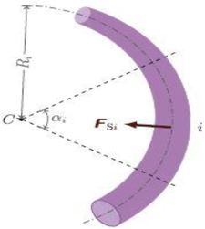
In addition to the surface tension parallel to the interface and perpendicular to the contour, due to the bending of the charged jet micro-element, an additional surface tension $F_{sn}^{i}$ is produced, and its line of action follows the radial direction of the corresponding curvature circle of the jet micro-element and points Center (Yarin and Zussman, 2004). At the same time, since the length of each segment of the jet micro-element is extremely small, the curvature radius of the curvature circle corresponding to the jet stream element segments of the (i-1)th, i-th, and (i + 1)-th segments is approximately equal. Therefore, the additional surface tension $F_{sn}^{i}$ is as shown in the formula (28).

(28)

F_{sn}^{i} = \frac{γ π d_{0} l_{0}^{\frac{1}{2}}}{4} [{(\frac{β_{i - 1}}{l_{i - 1}})}^{\frac{1}{2}} {sin}^{- 1} \frac{l_{i - 1}}{2 R_{i}} + {(\frac{β_{i + 1}}{l_{i + 1}})}^{\frac{1}{2}} {sin}^{- 1} \frac{l_{i + 1}}{2 R_{i}}] \frac{r_{c} - r_{i}}{|r_{c} - r_{i}|}

where:

R_{i}

is the radius of curvature of the curvature circle corresponding to the i-th, i-th, and i + 1-th segment jet micro-element segments; C is the center of the curvature circle;

r_{c}

is the vector radius of the center of the circle. Therefore, the resultant force

F_{si}

of the surface tension received by the straight segment of the i-th segment jet micro-element is as shown in the formula (29).

(29)

F_{si} = F_{s,i - 1}^{i} + F_{s,i + 1}^{i} + F_{sn}^{i} = \frac{γ π d_{0} l_{0}^{\frac{1}{2}}}{4} {\{(\frac{β_{i - 1}}{l_{i - 1}})}^{\frac{1}{2}} \frac{r_{i - 1} - r_{i}}{|r_{i - 1} - r_{i}|} + [{(\frac{β_{i - 1}}{l_{i - 1}})}^{\frac{1}{2}} {sin}^{- 1} \frac{l_{i - 1}}{2 R_{i}} + {(\frac{β_{i + 1}}{l_{i + 1}})}^{\frac{1}{2}} {sin}^{- 1} \frac{l_{i + 1}}{2 R_{i}}] \cdot \frac{r_{c} - r_{i}}{|r_{c} - r_{i}|} + {(\frac{β_{i + 1}}{l_{i + 1}})}^{\frac{1}{2}} {sin}^{- 1} \frac{l_{i + 1}}{2 R_{i}}\}

2.6

2.6 Air resistance

The charged jet will be subjected to the resistance of the air during the movement, and the resistance caused by the friction between the jet and the gas is equal to the sum of the frictional resistance and the differential pressure resistance (Yarin and Zussman, 2004). The frictional resistance is related to the shear stress in the boundary layer. The differential pressure resistance is related to the wake separated from the fluid surface by the flow line. The interference effect of the flow line depends on the shape of the fluid and the Reynolds number. The influence of the surface roughness is not considered in the model.

For the i-th segment jet micro-element straight line segment, see Fig. 3. it is also affected by the resistance $F_{f,i - 1}^{i}$ of the (i-1)-th segment jet micro-element segment and its resistance $F_{f,i + 1}^{i}$ of the (i + 1)-th segment jet micro-element segment. Therefore the air resistance $F_{fi}$ of the straight section of the i-th jet micro-element is as shown in Eq. (30).

(30)

F_{fi} = F_{f, i - 1}^{i} + F_{f, i + 1}^{i} = 6 μ_{a} π d_{0} l_{0}^{\frac{1}{2}} [{(\frac{β_{i - 1}}{l_{i - 1}})}^{\frac{1}{2}} |v_{i - 1}^{n} |+ {(\frac{β_{i + 1}}{l_{i + 1}})}^{\frac{1}{2}}| v_{i + 1}^{n}| + 6 μ_{a} (l_{i - 1} |v_{i - 1}^{t} |+ l_{i + 1}| v_{i + 1}^{t}|)]

where \{\begin{matrix} v_{i - 1}^{n} + v_{i - 1}^{t} = v_{i} \\ v_{i + 1}^{n} + v_{i + 1}^{t} = v_{i} \\ v_{i - 1}^{n} = \frac{v_{i} \cdot n_{i - 1}}{n_{i - 1} \cdot n_{i - 1}} \frac{r_{i - 1} - r_{i}}{|r_{i - 1} - r_{i}|} \\ n_{i - 1} = r_{i - 1} - r_{i} \\ v_{i + 1}^{n} = \frac{v_{i} \cdot n_{i + 1}}{n_{i + 1} \cdot n_{i + 1}} \frac{r_{i} - r_{i + 1}}{|r_{i} - r_{i + 1}|} \\ n_{i + 1} = r_{i} - r_{i + 1} \end{matrix}

where:

v_{i - 1}^{n}

v_{i - 1}^{t}

are the normal velocity and tangential velocity of the velocity segment of the i-th segment jet micro-element to the jet segment of the (i-1)th segment;

v_{i + 1}^{n}

and

v_{i + 1}^{t}

are the i-th segment jet respectively The velocity of the linear segment of the micro-element is projected onto the normal velocity and the tangential velocity of the (i + 1)-stage jet micro-element segment.

Section i, the effect of surface tension on the microelement section of a jet.

3 Calculation of governing equations

Through the force analysis described above, it is known that the straight segment of the i-th jet micro-element is affected by the electric field force $F_{Ei}$ , the Coulomb force $F_{Ci}$ , the viscoelastic force $F_{vi}$ , the surface tension $F_{si}$ , the air resistance $F_{fi}$ , and the gravity $G_{i}$ . Therefore, the resultant force $F$ of the i-th segment jet micro-line segment is as shown in Eq. (31).

(31)

F = F_{Ei} + F_{Ci} + F_{vi} + F_{si} + F_{fi} + G_{i}

According to Newton's second law, the resultant force of the straight segment of the i-th segment jet micro-element is equal to the first derivative of its momentum versus time, then Eq. (32) is obtained.

(32)

\begin{matrix} F = \frac{{dp}_{i}}{dt} = \frac{d (m_{i} v_{i})}{dt} = m_{i} \frac{{dv}_{i}}{dt} + v_{i} \frac{{dm}_{i}}{dt} \end{matrix}

The conservation of charge during the movement of a charged jet (Yarin and Zussman, 2004, (Yong et al., xxxx)gives the Eq. (33).

(33)

ρ_{q} π d_{i} |v_{i}| + k \frac{π d_{i}^{2}}{4} |E| = I

where:

k

is the dimensionless conductivity;

I

is the magnitude of the current. Because the charged jet fluid is not compressible, ie

\frac{\partial ρ}{\partial t} = 0

. According to the N-S equation in fluid mechanics, equation (34) is obtained.

(34)

ρ \frac{\partial v_{i}}{\partial t} + ρ (v_{i} \cdot \nabla) v_{i} = - \nabla p + μ_{i} \nabla^{2} v_{i} + ρ f

where:

\nabla p

represents the pressure gradient force acting on a unit volume of fluid;

ρ f

represents the mass force acting on a unit volume of fluid.

4 Numerical simulations

The results of numerical simulation of the jet by FLUENT software show that the motion state and trajectory of the jet can be observed obviously. From the simulation diagram of the jet trajectory, it can be found that the jet is mainly divided into stable section and unstable section. When the jet just left the needle, the electric field force on the jet was larger because of the strong electric field intensity at the needle and the uniform and stable distribution of the electric field. This will cause the jet to speed up continuously, and the trajectory of the jet is basically in a straight line. When the jet moves to a certain distance from the needle, the electric field intensity becomes weaker and the electric field force on the jet becomes smaller. Because of the interaction between jet charges, the jet will also be affected by the Kulun force. In addition, the jet is also affected by viscoelastic force, surface tension, air resistance and its own gravity. Therefore, these forces, together with the influence of external instability, will change the motion state of the jet immediately. Once the jet enters the unstable state, its motion will become more complicated, which will lead to the irregular curvilinear motion of the jet. In the process of jet movement in unstable section, because of the long track of jet motion and the constant volatilization of solvent, the diameter of jet is refined sufficiently, and finally the dry nanofibers are formed on the receiving device.

We might as well set the inlet velocity of the jet at the inlet boundary of the velocity to 30.0 m/s; Then five groups of data of rotation velocity of different air flow field were set up. The three groups of different rotation velocities were 60 rad/s, 120 rad/s, and 300 rad/s respectively. Therefore according to different parameter conditions, the corresponding trajectory simulation diagram of unstable jet can be obtained, as shown in Fig. 4.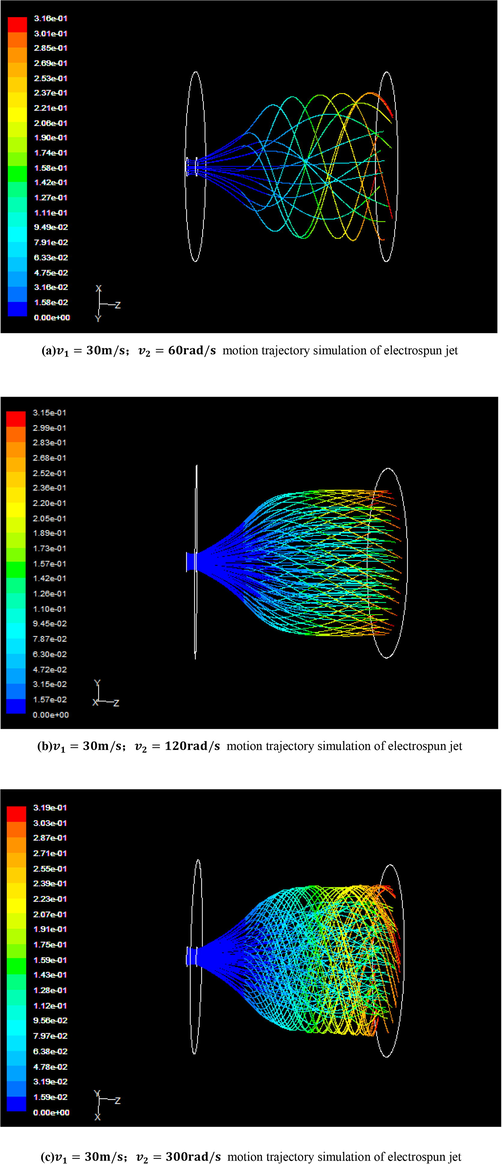

The simulation diagram of the jet trajectory.

From Fig. 4 it can be found that the jet is mainly divided into stable section and unstable section. When the jet just left the needle, the electric field force on the jet was larger because of the strong electric field intensity at the needle and the uniform and stable distribution of the electric field. This will cause the jet to speed up continuously, and the trajectory of the jet is basically in a straight line. When the jet moves to a certain distance from the needle, the electric field intensity becomes weaker and the electric field force on the jet becomes smaller. Because of the interaction between jet charges, the jet will also be affected by the Kulun force. In addition, the jet is also affected by viscoelastic force, surface tension, air resistance and its own gravity. Therefore, these forces, together with the influence of external instability, will change the motion state of the jet immediately. Once the jet enters the unstable state, its motion will become more complicated, which will lead to the irregular curvilinear motion of the jet. In the process of jet movement in unstable section, because of the long track of jet motion and the constant volatilization of solvent, the diameter of jet is refined sufficiently, and finally the dry nanofibers are formed on the receiving device.

5 Conclusion

(1)

Using Fink's first law, the mass transport equation of the solvent between the charged liquid jet and the surrounding gas medium is established. The behavioral model of viscoelastic fluid under different conditions is established, and the corresponding constitutive of viscoelastic fluid is obtained. Equation; using the principle of “mirror method”, the physical model of the applied electric field is established, and the electric field strength is qualitatively analyzed and quantitatively calculated.
(2)

Mechanical analysis of unstable segments of charged jets, including analysis and calculation of electric field force, Coulomb force, viscoelastic force, surface tension, air resistance and gravity.
(3)

Based on the force analysis, the coupled governing equations of the ideal behavior of charged jets in a three-dimensional Cartesian coordinate system are established.
(4)

From the simulation diagram of the jet trajectory, it can be found that the jet is mainly divided into stable section and unstable section, which is valid for the theory.

Acknowledgements

This work was partly supported by the Chang Jiang Youth Scholars Program of China and grants (51373033 and 11172064) from the National Science Foundation of China to Prof. Xiaohong Qin, As well as “The Fundamental Research Funds for the Central Universities” and “DHU Distinguished Young Professor Program” to her. It also has the support of the Key grant Project of Chinese Ministry of Education (No 113027A). This work has also been supported by “Sailing Project” from Science and Technology Commission of Shanghai Municipality (14YF1405100) to Dr. Hongnan Zhang.

References

Jianzong Zhang, . Numerical Simulation and Experimental Fitting of Electrospinning Jet Spinning Form. Shanghai: School of Science, Donghua University; 2012. p. :1-8.
Shin Y.M., Hohman M.M., Brenner M.P., . Experimental characterization of electrospinning: the electrically forced jet and instabilities. Polymer. 2001;42(25):9955-9967.
[Google Scholar]
Theron S.A., Yarin A.L., Zussman E., . Multiple jets in electrospinning: experiment and modeling. Polymer. 2005;46(9):2889-2899.
[Google Scholar]
Weiya Chen, Yanbo Liu, Yangzhi Wang, . Finite element analysis of electric field strength and distribution during multi-needle electrospinning. J. Textile Res.. 2014;7(06):1-6.
[Google Scholar]
Yarin A.L., Zussman E., . Upward needleless electrospinning of multiple nanofibers. Polymer. 2004;45(9):2977-2980.
[Google Scholar]
Yong Liang Zhi, Liang Deng Zong, Hong Qin Xiao, . Theoretical analysis and of three dimensional free surface of electrospinning. J. King Saud Univ. 2017
[Google Scholar]

Show Sections

[1] Jianzong Zhang, . Numerical Simulation and Experimental Fitting of Electrospinning Jet Spinning Form. Shanghai: School of Science, Donghua University; 2012. p. :1-8.

[2] Shin Y.M., Hohman M.M., Brenner M.P., . Experimental characterization of electrospinning: the electrically forced jet and instabilities. Polymer. 2001;42(25):9955-9967.
[Google Scholar]

[3] Theron S.A., Yarin A.L., Zussman E., . Multiple jets in electrospinning: experiment and modeling. Polymer. 2005;46(9):2889-2899.
[Google Scholar]

[4] Weiya Chen, Yanbo Liu, Yangzhi Wang, . Finite element analysis of electric field strength and distribution during multi-needle electrospinning. J. Textile Res.. 2014;7(06):1-6.
[Google Scholar]

[5] Yarin A.L., Zussman E., . Upward needleless electrospinning of multiple nanofibers. Polymer. 2004;45(9):2977-2980.
[Google Scholar]

[6] Yong Liang Zhi, Liang Deng Zong, Hong Qin Xiao, . Theoretical analysis and of three dimensional free surface of electrospinning. J. King Saud Univ. 2017
[Google Scholar]

Force analysis of unstable section of electrostatic spinning charged jet

Abstract

Keywords

Electrostatic spinning

Charged jet

Rapid whipping

Viscoelastic behavior model

Mechanical analysis

1 Introduction

1.1 Hypothesis and establishment of a mechanical model for unstable segments with charged jets

1.2 Mass transport equation of solvent between charged jet and surrounding gaseous medium

1.3 Visco-elastic behavior model and constitutive equation of charged jet

1.4 Calculation of applied electric field strength

2 Mechanical analysis of the micro-element of unstable jet volume

2.1 Gravity

2.2 Applied electric field force

2.3 Coulomb force

2.4 Viscoelastic force

2.5 Surface tension

2.6 Air resistance

3 Calculation of governing equations

4 Numerical simulations

5 Conclusion

Acknowledgements

References

Suggested read for related articles: