Decomposed channel based Multi-Stream Ensemble: Improving consistency targets in semi-supervised 2D pose estimation

Jiaqi Wu; Junbiao Pang; Qingming Huang

doi:10.1016/j.jksus.2023.103078

View/Download PDF

Buy Reprints

PDF

Translate this page into:

Full Length Article

03 2023

:36;

103078

doi:

10.1016/j.jksus.2023.103078

Decomposed channel based Multi-Stream Ensemble: Improving consistency targets in semi-supervised 2D pose estimation

Jiaqi Wu^{^a}, Junbiao Pang^{^a,⁎}, Qingming Huang^{^b}

a Beijing University of Technology Beijing, China

b University of Chinese Academy of Sciences Beijing, China

⁎Corresponding author at: Beijing University of Technology Beijing, China. Junbiao_pang@bjut.edu.cn (Junbiao Pang),

Received: 2023-8-19, Accepted: 2023-12-21,

Disclaimer:
This article was originally published by Elsevier and was migrated to Scientific Scholar after the change of Publisher.

Abstract

Objectives

In pose estimation, semi-supervised learning is a crucial approach to overcome the lack of information problem of labeled data. However, for semi-supervised learning, the insufficient number of labeled samples also severely affects its functionality. The fewer labeled the data, the less stable the prediction. Deep ensemble is a good way to improve model accuracy and stability. However, the training time of model ensemble is long and the resource consumption is high, so it cannot be applied in many practical scenarios. Therefore, the methods we propose the Decomposed Channel based Multi-Stream Ensemble (DCMSE) network, which can extend a single model to a stream-ensemble structure and generate the ensemble prediction to solve the large variance of prediction from the lack of labeled data, and improve the performance. The Channel Deconstruction and Ensembling (CDE) module makes the network benefits from both diversity and commonality by implementing ensemble without increasing the size of parameters. The output features are split into two parts, common-channels and private-channels. In feature sampling, on the one hand, common channels can provide commonality between streams. On the other hand, private channels can provide diversity for each stream and avoid homogenization of the predictions for each stream. Both diversity and commonality allow the network to not only gain in the ensemble of streams, but also improve the prediction accuracy of each stream itself.

Results

Moreover, we propose mean-stream consistency constraints and cross-stack consistency constraints to obtain gains from unlabeled data. The Mean-Stream (MS) consistency constraint uses multi-stream ensemble prediction to additionally supervise each stream. Based on the characteristics of the Stacked Hourglass model, the Cross-Stage consistency constraint (CS) uses the forecasting results of later stages to supervise the forecasting of previous stages from the perspective of stages.

Conclusion

Our approach achieves better results than SOTAs on the FLIC and Openfield-Pranav and our Sniffing data-set. Specifically, on the MSE, our method achieves at least 0.88, 0.13, and 0.08 improvements over the SOTA method on the FLIC, Openfield-Pranav, and our Sniffing datasets, respectively.

Keywords

Multi-Stream Ensemble

UDA-AP

Openfield-Pranav

DCMSE network

CDE module

Show Related Articles from PubMed

1 Introduction

Pose estimation is an essential subject in computer vision, and it has achieved many outstanding results, such as (Newell et al., 2016; Sun et al., 2019; Tompson et al., 2014; Wei et al., 2016; Xiao et al., 2018 ). All the above methods achieve excellent results with sufficient labeled data. However, these methods are highly sensitive to the amount of labeled data. Manual annotation of poses is complex and costly. Therefore, reducing the amount of labeled data has become a focus of research.

Currently, unsupervised pose estimation based on transfer learning has achieved exciting results. The main idea of UDA-AP (Li et al., 2021) is to gain knowledge from synthetic animal data and apply this knowledge to target domain recognition using transfer learning. However, due to the great difficulty of pose estimation, when the difference between source and target domains is large, a few of labeled data is still needed to guide the model training. Therefore, semi-supervised pose estimation based on few labeled samples still plays an essential role.

The main role of semi-supervised learning is to use a small amount of labeled data and a large amount of unlabeled data simultaneously, so that the model can achieve better predictive performance. Currently, semi-supervised learning methods are mainly applied to classification tasks. In general, there are two categories of semi-supervised learning: consistency-based and pseudo-label-based method.

The idea of consistency-based methods (Berthelot et al., 2019; Laine and Aila, 2016; Sajjadi et al., 2016; Sohn et al., 2020; Tarvainen and Valpola, 2017 ) is that the model should have consistent predictions for different augmented samples of the same sample. Therefore, the main approach of such methods is to construct long-term stable and effective consistency-based supervision, thereby obtaining additional supervision from unlabeled data.

In pseudo-label-based methods (Arazo et al., 2020; Berthelot et al., 2019; Lee et al., 2013; Radosavovic et al., 2018; Wang et al., 2018; Xie et al., 2020; Zhai et al., 2019 ), an initial model is first trained using labeled data, and then use the initial model predicts the unlabeled data to generate pseudo-labels. Finally, using pseudo-labels to train the initial model itself. The bottleneck of this approach is that the quality of the generated pseudo-labels deeply depends on the initial model, and the noise of the pseudo-labels can easily degrade the model performance.

In the above semi-supervised methods, the model predictions are prone to fluctuation when there is less labeled data. The less labeled data, the less stable the prediction. As shown in Fig. 1, the predictions of single-model-based methods are prone to fluctuations and have large variance. This can lead to a reduction in accuracy. In extreme cases, the semi-supervised framework breaks down, as the model fails to provide valid predictions. The model collapse mentioned in (Xie et al., 2021) occurs, that is, the prediction accuracy of semi-supervised learning is lower than that of supervised one.Fig. 2.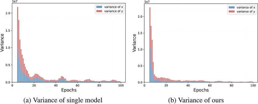

The variance of single-model and our model.

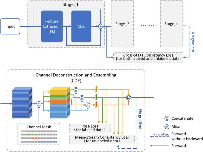
Overview of the proposed Decomposed Channel based Multi-Stream Ensemble (DCMSE) network.

In this work, we propose a “no-cost” stream-based ensemble method to solve the problem of unstable prediction, in the case of few labeled data. The Channel Deconstruction and Ensembling (CDE) can sample the output features on the channel dimension, form multiple different features, and predict them through the corresponding FC layer. The output features are split into two parts, common-channels and private-channels. In feature sampling, on the one hand, the common channel can provide commonality between streams. On the other hand, the private channels can provide diversity for each stream and avoid the homogenization of the predictions of each stream. Both diversity and commonality can not only make the network gain in stream ensembling, but also improves the prediction accuracy of each stream itself.

In addition, we propose two consistency constraints to further improve the accuracy of the ensemble prediction of multiple stream. The Mean-Stream (MS) consistency constraint uses multi-stream ensemble prediction to additionally supervise each stream. Based on the characteristics of the Stacked Hourglass model, the Cross-Stage consistency constraint (CS) uses the forecasting results of later stages to supervise the forecasting of previous stages from the perspective of stages. The project code and Sniffing dataset are publicly available on https://github.com/Qi2019KB/DCMSE/tree/master.

2 Summary of our main contributions

We propose a simple structure, named Decomposed Channels based Multi-Stream Ensemble (DCMSE), to extend a model to an ensemble form easily. In DCMSE, the private channel groups of each stream can improve the diversity, which can accelerate the performance of multi-stream ensemble. Moreover, the co-channel group allows the model to learn common features from all streams, which can improve the performance of each stream itself.
We propose the Mean-Stream Consistency Loss based on the multi-stream ensemble and the Cross-Stage Consistency Loss based on the cascade structure of the pose estimation model. Both of them allow the model to efficiently gain additional supervision from unlabeled data.
With a few labeled data, our method achieves better results than the state-of-art pose estimation method. We implemented this result on the public data-set FLIC (Sapp and Taskar, 2013), Openfield-Pranav (Mathis et al., 2018), and our own Sniffing data-set.

3 Related work

Semi-supervised learning. Semi-supervised learning (SSL) (Higuchi et al., 2022; Li et al., 2022; Njima et al., 2022; Xu et al., 2022) focus on reducing the need for labeled data. The main idea is to use a small amount of labeled data and a large amount of unlabeled data simultaneously, so that the model can achieve better predictive performance. In general, there are two categories of semi-supervised learning.

One popular approach is based on the pseudo-labeling (Arazo et al., 2020; Lee et al., 2013; Radosavovic et al., 2018 ). Labeled data is used to train initial model as per-trained model, and the model generates pseudo-labels from unlabeled data, then the model is trained with artificial labels and pseudo-labels. Another one is the consistency regularization. It encourages the model have consistent predictions for different augmented samples of the same sample.

Deep Ensemble. Training multiple deep neural networks (DNNs) is to improve the predictive performance. Wang et al., 2021 is to average the parameters stored at multiple checkpoints to obtain a new model. The advantage of this ensemble approach is that the training cost is low, but the prediction accuracy barely increases due to the lack of diversity.

Another approach is to ensemble multiple deep models and take the average prediction as the final output. This approach can improve performance, but is costly to train.

4 Method

4.1

4.1 2D pose estimation with Multi-Stage model

In 2D Pose estimation, the main task is to predict the accurate position of $K$ key points which are predefined manually in the input Image $I$ . Most recent approaches transform this problem into predicting $K$ Gaussian heat-maps $H$ that encode the probability of each key point at each spatial location in $I$ . Therefore, a Gaussian kernel function is used to transform the coordinate values into Gaussian heat maps, where one key point corresponds to one heat-map, and the heat maps are used as ground-truth for model training. During prediction, the location with the highest response value is selected from the heat-map generated by the model as the predicted location of the key point. Denote the labeled training data-set as $L = {\{(I^{l}, H^{l})\}}_{l = 1}^{N^{L}}$ . To train the 2D pose estimation model $f (\cdot, θ)$ , we write simply $f (\cdot)$ . we minimize the MSE loss between the prediction and ground-truth heat map. Therefore, the Pose loss, as $L_{pose}$ , can be expressed as:

(1)

L_{pose} = E_{I \in L} ‖ f (I) - H ‖^{2},

The $M$ stage pose estimation model $g (\cdot, θ)$ , we write simply $g (\cdot)$ , such as Stacked Hourglass (Newell et al., 2016), stacks multiple modules with the same structure end to end, and feeds the previous model’s predictions and features to the next. There is supervised learning at each stage, called intermediate supervision, to ensure performance at each stage. So, for image $I$ , the input $X_{m}^{I}$ of the $m$ -th stage can be expressed as:

(2)

X_{m}^{I} = \{\begin{matrix} I & m = 1 \\ I + P_{m - 1}^{I} + φ_{m - 1}^{I} & otherwise, \end{matrix}

where

P_{m - 1}^{I} = g_{m - 1} (X_{m - 1}^{I})

is the prediction in the

(m - 1)

-th stage of the model

g (\cdot)

φ_{m - 1}^{I}

is the feature extracted by the feature extraction module in the

(m - 1)

-th stage of the model

g (\cdot)

4.2

4.2 Channel Deconstruction and ensembling

In each stage of the multi-stage network, the Channel Deconstruction and Ensembling (CDE) module is located behind the feature extraction (FE) module. The CDE deconstructs the features extracted by FE in the channel dimension and forms $n$ new features corresponding to $n$ streams. We assume that the feature extracted from a sample by the FE is of $C \times H \times W$ dimension, where $H$ , $W$ , $C$ denote the height, width and number of channels, respectively. Specifically, the CDE extracts $n$ features with channel $C^{'}$ from the C-channels in the input feature according to the splitting factor $α$ as the private features of streams. The feature corresponding to the remaining channels is treated as common feature and shared by all streams. Each private feature is concatenated with the common feature and passed to the regressor of each stream for prediction. In the $m$ -th stage, consider the ensemble output ${\tilde{P}}_{m}^{I}$ of the image $I$ by averaging each stream’s prediction $P_{m, n}^{I}$ , i.e.,

(3)

{\tilde{P}}_{m}^{I} = \frac{1}{n} \sum_{n = 1}^{N} P_{m, n}^{I},

At the same time, we pass the full features extracted by feature extraction module with the ensemble output to the next stage. So, for image $I$ , the input $X_{m}^{I}$ of the $m$ -th stage can be rewritten as:

(4)

X_{m}^{I} = \{\begin{matrix} I & m = 1 \\ I + {\tilde{P}}_{m - 1}^{I} + φ_{m - 1}^{I} & otherwise, \end{matrix}

4.3

4.3 Mean-Stream consistency constraint

The $M$ stage pose estimation model $g (\cdot)$ also learns about unlabeled data. Denote the unlabeled training data-set as $U = {\{I^{u}\}}_{u = 1}^{N^{U}}$ .

Several studies (Ren et al., 2016; Zhang and Suganthan, 2017) have demonstrated that the performance of a single model is inferior than that of an ensemble of models. Therefore, in each stage, we minimize the MSE loss between the ensemble output and each stream’s prediction. Denote the prediction of the $n$ -th stream to sample $I, I \in U$ in the $m$ -th stage as $P_{m, n}^{I}$ , the ensemble output to sample $I, I \in U$ in the $m$ -th stage as ${\tilde{P}}_{m}^{I}$ . Therefore, the mean-stream consistency loss, as $L_{ms}$ , can be expressed as:

(5)

L_{ms} = \frac{1}{m} \frac{1}{n} \sum_{m = 1}^{M} \sum_{n = 1}^{N} E_{I \in U} ‖ P_{m, n}^{I} - {\tilde{P}}_{m}^{I} ‖^{2},

Note that the consistency constraint affects both parties. To avoid a negative effect on the model performance, we compute this loss using a replica of the ensemble output with the gradient information removed, so that the model is not updated from the ensemble output.

4.4

4.4 Cross-Stage consistency constraint

As stated in Newell et al., 2016, in multi-stage pose estimation model, subsequent stages allow the high-level features, extracted by previous stage, to be processed again to make the network to best refine predictions. Moreover, the more accurate the prediction at the front stage, the more accurate the prediction at the back stage, which is in line with the goal of intermediate supervision. Therefore, we minimize the MSE loss between the ensemble output of the first stage and the ensemble output of the last stage. Therefore, the cross-stage consistency loss, as $L_{cs}$ , can be expressed as:

(6)

L_{cs} = E_{I \in (L \cup U)} ‖ {\tilde{P}}_{1}^{I} - {\tilde{P}}_{m}^{I} ‖^{2},

Note that the cross-stage consistency constraint can work on both labeled and unlabeled data. For the same reason as in $L_{ms}$ , we compute this loss using a replica of the final-stage ensemble output with the gradient information removed.

4.5

4.5 Total loss

We summarize the objective function as follows:

(7)

L = λ_{pose} L_{pose} + λ_{ms} L_{ms} + λ_{cs} L_{cs},

where

λ_{pose}

λ_{ms}

λ_{cs}

are the weights to balance all losses.

5 Experiment

We evaluate our model on three datasets. FLIC (Sapp and Taskar, 2013) data-set, an public human pose data-set; Openfield-Pranav (Mathis et al., 2018) data-set, an public mouse data-set; Sniffing data-set, a mouse data-set collected by ourselves.

5.1

5.1 Implementation details

We use Stacked Hourglass (Newell et al., 2016) with a stack number of 3 as the pose estimation model. When the CDE is created, the number of streams, $N$ , is 3 and the splitting factor, $α$ , is 0.2.

All input images are resized to $256 \times 256$ pixels. And we use the data augmentation that includes random rotation ( $+ / - 30$ degrees), and random scaling ( $0.75 - 1.25$ ) and random horizontal flip.

The initial value of $λ_{pose}$ is the constant 10. The initial value of $λ_{ms}$ is 0 and after 50 epochs rises to a maximum of 50. The initial value of $λ_{cs}$ is 0 and after 50 epochs rises to a maximum of 5.

5.2

5.2 FLIC dataset

The FLIC (Sapp and Taskar, 2013) dataset is a publicly available human pose dataset consisting of 5003 images taken from movies, including 3987 training data and 1016 test data.

The MSE and PCK@0.2 are reported (see results in Fig. 3 and Table 1).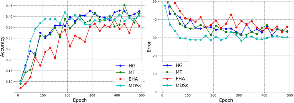

Comparison to the baselines with 500 training samples with 30% labeled data on the FLIC dataset. Supervised learning is training with Newell et al., 2016. And, DNCL (Shi et al., 2018), Mean Teacher (Tarvainen and Valpola, 2017), ESCP (Xie et al., 2021) and ours are semi-supervised learning.

Table 1 Comparison to the baselines on the FLIC dataset. The 500*0.3 means that there are 500 samples in the training set, of which 30% are labeled samples and 70% are unlabeled samples.

Method	*5000.3**		*5000.5**
Method	MSE	PCK@0.2	MSE	PCK@0.2
HG (Newell et al., 2016)	37.27	0.436	33.36	0.516
DNCL (Shi et al., 2018)	35.56	0.456	30.22	0.535
MT (Tarvainen and Valpola, 2017)	35.58	0.448	28.68	0.551
ESCP (Xie et al., 2021)	39.57	0.390	35.06	0.486
Ours	32.26	0.490	27.80	0.574

5.3

5.3 Openfield-Pranav data-set

The Openfield-Pranav data-set is a publicly available mouse data-set consisting of 1000 images with one instance per image.

The MSE and PCK@0.2 are reported (see results in Fig. 4 and Table 2). Our method achieves the best results on the Openfield-Pranav dataset in both cases 100*0.3 and 100*0.5, and the increase amount is 1.8 % and 0.7 % respectively.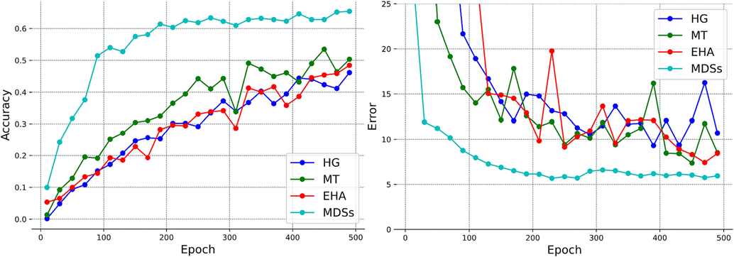

Error and accuracy curves for each baseline with 100 training samples with 30% labeled data on the Openfield-Pranav dataset.

Table 2 Comparison to the baselines on the Openfield-Pranav dataset. 100*0.3 means that there are 100 training samples and 30% of them are labeled.

Method	*1000.3**		*1000.5**
Method	MSE	PCK@0.2	MSE	PCK@0.2
HG	8.54	0.565	4.34	0.725
DNCL	5.56	0.647	4.13	0.756
MT	5.89	0.635	4.36	0.739
ESCP	5.87	0.617	4.25	0.717
Ours	5.50	0.665	4.00	0.763

5.4

5.4 Sniffing dataset

The Sniffing dataset was captured by ourselves from real experimental environments. The MSE and PCK@0.2 are reported (see results in Fig. 5 and Table 3). Our method achieves the best results on the Sniffing dataset in both cases 100*0.3 and 100*0.5, and the increase amount is 0.9 % and 0.3 % respectively.

Error and accuracy curves for each baseline with 100 training samples with 30% labeled data on the Sniffing dataset.

Table 3 Comparison to the baselines on our Sniffing Data-set. 100*0.3 means that there are 100 training samples and 30% of them are labeled.

Method	*1000.3**		*1000.5**
Method	MSE	PCK@0.2	MSE	PCK@0.2
HG	5.18	0.602	4.26	0.663
DNCL	4.47	0.634	3.89	0.698
MT	4.73	0.613	4.14	0.676
ESCP	5.03	0.596	3.93	0.675
Ours	4.26	0.643	3.81	0.701

6 Ablation study

We perform ablation studies on the FLIC and Openfield-Pranav datasets.

In the CDE ablation experiments, we evaluate the role of CDE in terms of ensembling. We construct two simple models. HG-Ensemble is a simple parallel ensembling of the Stacked Hourglass (HG), taking the average predicted values of three HG as the output of the entire model. In addition, we remove the CDE module from our network (stream count is 3), which means that the regressors of all three streams share the same features as the input. Finally, we use Stacked Hourglass for supervised learning and evaluate their predictive performance.

As shown in Table 4, our network achieved significant performance gains despite the removal of CDE. This is because the prediction accuracy of the regressors for each stream in our network is significantly improved compared to HG-Ensemble. Multiple streams share the same feature, so that the feature extraction module in the network can learn to extract the common feature of higher dimensions, which can improve the accuracy of each stream’s regress.

Table 4 The result of Openfield-Pranav dataset. The CDE is evaluated from an ensemble perspective. Stream Predictions is a list of the prediction performance of all streams.

Method	Stream Count	MSE	PCK@0.2	Stream’s Predictions
Method	Stream Count	MSE	PCK@0.2	MSE	PCK@0.2
Supervised	–	6.78	0.571	–	–
HG-Ensemble	3	6.34	0.600	7.30, 6.99, 8.74	0.569, 0.574, 0.553
Ours (without CDE)	3	5.89	0.637	5.94, 5.92, 5.95	0.626, 0.628, 0.625

We also performed ablation experiments on the Mean-Stream(MS) and Cross-Stage (CS) consistency constraint, shown in Table 5.

Table 5 The ablation experiments on the Mean-Stream (MS) and Cross-Stage (CS) consistency constraint. “Y” and “N” mean “using” and “not using”, respectively.

Method	Dataset	MS	CS	MSE	PCK@0.2
Ours	FLIC 100*0.3	N	N	45.91	0.284
		Y	N	45.47	0.288
		Y	Y	44.42	0.297
	Openfield-Pranav 100*0.3	N	N	6.28	0.643
		Y	N	5.88	0.651
		Y	Y	5.68	0.665

7 Discussions

After completing the above experiments and proving the effectiveness of our method, we discuss two important parameters of the CDE module: the stream count $N$ and the splitting factor $α$ . We put different values on each of these variables and see what they do. The experimental results are shown in Table 6.

Table 6 Compare the influence of different values of stream count

N

and splitting factor

α

on the model performance.

Method	Stream Count	Splitting Factor	MSE	PCK@0.2	Stream’s Predictions
Method	Stream Count	Splitting Factor	MSE	PCK@0.2	MSE	PCK@0.2
Ours	3	0.1	6.22	0.629	6.28, 6.26, 6.25	0.618, 0.623, 0.622
	3	0.15	5.78	0.637	5.82, 5.84, 5.84	0.632, 0.627, 0.634
	3	0.2	5.78	0.648	5.78, 5.90, 5.83	0.641, 0.644, 0.638
Ours	2	0.2	6.41	0.630	6.45, 6.45	0.620, 0.623
	3	0.2	5.85	0.657	5.73, 5.98, 6.00	0.640, 0.643, 0.648
	4	0.2	5.92	0.645	6.00, 6.00, 6.00, 6.01	0.630, 0.629, 0.634, 0.631

First, we fix the stream count $N$ to 3 and set the splitting factor $α$ to 0.1, 0.15 and 0.2, respectively. It can be seen that the prediction performance of the model gradually improves as the splitting factor increases.This indicates that more private features contribute to the increase of the ensembling performance.

Then, we fix the splitting factor $α$ to 0.2 and set the stream count $N$ to 2, 3 and 4, respectively. The results show that more streams are not always better. This is because when the number of streams increases, the size of the common features decreases, which adversely affects the model. Therefore, we need to balance these two parameters. In all experiments, we used this optimal set of parameters.

8 Conclusion

The DCMSE offers a practical and efficient solution to enhance the accuracy and stability of semi-supervised learning when labeled data is scarce. Its adaptability and superior performance make it a promising tool for a wide range of real world applications. Semi-supervised learning is a crucial approach to address the absence of labeled data, the insufficient number of labeled samples also severely affects its functionality. Model ensembles are a useful way to improve model accuracy and stability. However, model ensembles suffer from lengthy training times and extreme resource consumption, so they cannot be applied in many real-world scenarios. The main aim of our study is to build an ensemble prediction framework at a lower cost and use ensemble prediction to address inaccuracies and instabilities in semi-supervised learning when labeled data is insufficient.

The DCMSE network transforms the traditional model ensemble idea into a flow ensemble inside the model. On the one hand, it creates the multi-branch structure needed for ensemble prediction. On the other hand, it does not increase the number of model parameters due to the feature sample-based ensemble of streams. Therefore, it is easy to generalize to different tasks and to different models. With few labeled data, our method achieves better results than state-of-the-art pose estimation methods. We implement this result on the public datasets FLIC, Openfield-Pranav, and our own Sniffing dataset. In terms of MSE, our method achieves at least 0.88, 0.13 and 0.08 improvement over the SOTA method on FLIC, Openfield-Pranav and our Sniffing dataset, respectively.

Consent to Participate.

Informed consent was obtained from all individual participants included in the study.

Consent to Publish.

The participant has consented to the submission in this Journal.

Ethical approval.

This article does not contain any studies with human participants or animals performed by any of the authors.

Fund statement.

There is no funding for this research.

Author’s contributions.

Jiaqi Wu made the primary contribution to this study, which included the design and methodology of this study, the evaluation of the results, and the writing of the manuscript. Junbiao Pang and Qingming Huang contributed to the methodology of this study.

Declaration of Competing Interest

The authors declare that they have no known competing financial interests or personal relationships that could have appeared to influence the work reported in this paper.

References

Eric Arazo, Diego Ortego, Paul Albert, Noel E O’Connor, and Kevin McGuinness. Pseudo-labeling and confirmation bias in deep semi-supervised learning. In: 2020 International Joint Conference on Neural Networks (IJCNN), pages 1–8. IEEE, 2020. 1, 2.
Berthelot D., Carlini N., Goodfellow I., Papernot N., Oliver A., Raffel C.A., . Mixmatch: A holistic approach to semi-supervised learning. Adv. Neural Inf. Proces. Syst.. 2019;32:1.
[Google Scholar]
David Berthelot, Nicholas Carlini, Ekin D Cubuk, Alex Kurakin, Kihyuk Sohn, Han Zhang, and Colin Raffel. Remixmatch: Semi-supervised learning with distribution alignment and augmentation anchoring. arXiv preprint arXiv:1911.09785, 2019. 1.
Chen Li and Gim Hee Lee. From synthetic to real: Unsupervised domain adaptation for animal pose estimation. In: Proceedings of the IEEE/CVF Conference on Computer Vision and Pattern Recognition, pages 1482–1491, 2021. 1.
Higuchi Yosuke, Moritz Niko, Le Roux Jonathan, Hori Takaaki, . Momentum pseudo-labeling: Semi-supervised asr with continuously improving pseudo-labels. IEEE J. Sel. Top. Signal Process.. 2022;16(6):1424-1438.
[Google Scholar]
Samuli Laine and Timo Aila. Temporal ensembling for semi-supervised learning. arXiv preprint arXiv:1610.02242, 2016. 1, 2.
Dong-Hyun Lee et al. Pseudo-label: The simple and efficient semi-supervised learning method for deep neural networks. In Workshop on challenges in representation learning, ICML, volume 3, page 896, 2013. 1, 2.
Hengduo Li, Zuxuan Wu, Abhinav Shrivastava, and Larry S Davis. Rethinking pseudo labels for semi-supervised object detection. In Proceedings of the AAAI Conference on Artificial Intelligence, volume 36, pages 1314–1322, 2022. 2.
Alexander Mathis, Pranav Mamidanna, Kevin M Cury, Taiga Abe, Venkatesh N Murthy, Mackenzie Weygandt Mathis, and Matthias Bethge. Deeplabcut: markerless pose estimation of user-defined body parts with deep learning. Nature neuroscience, 21(9):1281–1289, 2018. 1, 2, 5, 6, 7.
Alejandro Newell, Kaiyu Yang, and Jia Deng. Stacked hourglass networks for human pose estimation. In: European conference on computer vision, pages 483–499, 2016. 1, 2, 4, 5, 6, 8.
Njima W., Bazzi A., Chafii M., . Dnn-based indoor localization under limited dataset using gans and semi-supervised learning. IEEE Access. 2022;10(69896–69909):2.
[Google Scholar]
Ilija Radosavovic, Piotr Dolĺar, Ross Girshick, Georgia Gkioxari, and Kaiming He. Data distillation: Towards omni-supervised learning. In: Proceedings of the IEEE conference on computer vision and pattern recognition, pages 4119–4128, 2018. 1, 2.
Ren Y.e., Zhang L.e., Suganthan P.N., . Ensemble classification and regression-recent developments, applications and future directions. IEEE Comput. Intell. Mag.. 2016;11(1):41-53. 4
[Google Scholar]
Sajjadi M., Javanmardi M., Tasdizen T., . Regularization with stochastic transformations and perturbations for deep semi-supervised learning. Adv. Neural Inf. Proces. Syst.. 2016;29:1.
[Google Scholar]
Ben Sapp and Ben Taskar. Modec: Multimodal decomposable models for human pose estimation. In: Proceedings of the IEEE conference on computer vision and pattern recognition, pages 3674–3681, 2013. 1, 2, 5, 6, 7.
Sohn K., Berthelot D., Carlini N., Zhang Z., Zhang H., Raffel C.A., Cubuk E.D., Kurakin A., Li C.-L., . Fixmatch: Simplifying semi-supervised learning with consistency and confidence. Adv. Neural Inf. Proces. Syst.. 2020;33(596–608):1.
[Google Scholar]
Ke Sun, Bin Xiao, Dong Liu, and Jingdong Wang. Deep high-resolution representation learning for human pose estimation. In: Proceedings of the IEEE/CVF conference on computer vision and pattern recognition, pages 5693–5703, 2019. 1.
Tarvainen Antti, Valpola Harri, . Mean teachers are better role models: Weight-averaged consistency targets improve semi-supervised deep learning results. Adv. Neural Inf. Proces. Syst.. 2017;30 1, 2, 5, 6
[Google Scholar]
Tompson J.J., Jain A., LeCun Y., Bregler C., . Joint training of a convolutional network and a graphical model for human pose estimation. Adv. Neural Inf. Proces. Syst.. 2014;27:1.
[Google Scholar]
Keze Wang, Xiaopeng Yan, Dongyu Zhang, Lei Zhang, and Liang Lin. Towards human-machine cooperation: Selfsupervised sample mining for object detection. In Proceedings of the IEEE Conference on Computer Vision and Pattern Recognition, pages 1605–1613, 2018. 1.
Wang F., Wei G., Liu Q., Jinxiang O.u., Lv H., . Boost neural networks by checkpoints. Adv. Neural Inf. Proces. Syst.. 2021;34(19719–19729):3.
[Google Scholar]
Shih-En Wei, Varun Ramakrishna, Takeo Kanade, and Yaser Sheikh. Convolutional pose machines. In Proceedings of the IEEE conference on Computer Vision and Pattern Recognition, pages 4724–4732, 2016. 1, 2.
Bin Xiao, Haiping Wu, and Yichen Wei. Simple baselines for human pose estimation and tracking. In Proceedings of the European conference on computer vision (ECCV), pages 466–481, 2018. 1.
Qizhe Xie, Minh-Thang Luong, Eduard Hovy, and Quoc V Le. Self-training with noisy student improves imagenet classification. In Proceedings of the IEEE/CVF conference on computer vision and pattern recognition, pages 10687–10698, 2020. 1.
Rongchang Xie, Chunyu Wang, Wenjun Zeng, and Yizhou Wang. An empirical study of the collapsing problem in semi-supervised 2d human pose estimation. In Proceedings of the IEEE/CVF International Conference on Computer Vision, pages 11240–11249, 2021. 2, 3, 5, 6.
Xiaohua Zhai, Avital Oliver, Alexander Kolesnikov, and Lucas Beyer. S4l: Self-supervised semi-supervised learning. In: Proceedings of the IEEE/CVF International Conference on Computer Vision, (pages 1476–1485), 2019. 1.
Zhang L.e., Suganthan P.N., . Benchmarking ensemble classifiers with novel Co-trained kernel ridge regression and random vector functional link ensembles [research frontier] IEEE Comput. Intell. Mag.. 2017;12(4):61-72.
[Google Scholar]

Appendix A

Supplementary data

Supplementary data to this article can be found online at https://doi.org/10.1016/j.jksus.2023.103078.

Appendix A

Supplementary data

The following are the Supplementary data to this article:

Supplementary data 1

Download

Introduction

Summary of our main contributions

Related work

Method

2D pose estimation with Multi-Stage model
Channel Deconstruction and ensembling
Mean-Stream consistency constraint
Cross-Stage consistency constraint
Total loss

Experiment

Implementation details
FLIC dataset
Openfield-Pranav data-set
Sniffing dataset

Ablation study

Discussions

Conclusion

Fulltext Views
3

PDF downloads
0

View/Download PDF
Download Citations

BibTeX
RIS

Show Sections

[1] Eric Arazo, Diego Ortego, Paul Albert, Noel E O’Connor, and Kevin McGuinness. Pseudo-labeling and confirmation bias in deep semi-supervised learning. In: 2020 International Joint Conference on Neural Networks (IJCNN), pages 1–8. IEEE, 2020. 1, 2.

[2] Berthelot D., Carlini N., Goodfellow I., Papernot N., Oliver A., Raffel C.A., . Mixmatch: A holistic approach to semi-supervised learning. Adv. Neural Inf. Proces. Syst.. 2019;32:1.
[Google Scholar]

[3] David Berthelot, Nicholas Carlini, Ekin D Cubuk, Alex Kurakin, Kihyuk Sohn, Han Zhang, and Colin Raffel. Remixmatch: Semi-supervised learning with distribution alignment and augmentation anchoring. arXiv preprint arXiv:1911.09785, 2019. 1.

[4] Chen Li and Gim Hee Lee. From synthetic to real: Unsupervised domain adaptation for animal pose estimation. In: Proceedings of the IEEE/CVF Conference on Computer Vision and Pattern Recognition, pages 1482–1491, 2021. 1.

[5] Higuchi Yosuke, Moritz Niko, Le Roux Jonathan, Hori Takaaki, . Momentum pseudo-labeling: Semi-supervised asr with continuously improving pseudo-labels. IEEE J. Sel. Top. Signal Process.. 2022;16(6):1424-1438.
[Google Scholar]

[6] Samuli Laine and Timo Aila. Temporal ensembling for semi-supervised learning. arXiv preprint arXiv:1610.02242, 2016. 1, 2.

[7] Dong-Hyun Lee et al. Pseudo-label: The simple and efficient semi-supervised learning method for deep neural networks. In Workshop on challenges in representation learning, ICML, volume 3, page 896, 2013. 1, 2.

[8] Hengduo Li, Zuxuan Wu, Abhinav Shrivastava, and Larry S Davis. Rethinking pseudo labels for semi-supervised object detection. In Proceedings of the AAAI Conference on Artificial Intelligence, volume 36, pages 1314–1322, 2022. 2.

[9] Alexander Mathis, Pranav Mamidanna, Kevin M Cury, Taiga Abe, Venkatesh N Murthy, Mackenzie Weygandt Mathis, and Matthias Bethge. Deeplabcut: markerless pose estimation of user-defined body parts with deep learning. Nature neuroscience, 21(9):1281–1289, 2018. 1, 2, 5, 6, 7.

[10] Alejandro Newell, Kaiyu Yang, and Jia Deng. Stacked hourglass networks for human pose estimation. In: European conference on computer vision, pages 483–499, 2016. 1, 2, 4, 5, 6, 8.

[11] Njima W., Bazzi A., Chafii M., . Dnn-based indoor localization under limited dataset using gans and semi-supervised learning. IEEE Access. 2022;10(69896–69909):2.
[Google Scholar]

[12] Ilija Radosavovic, Piotr Dolĺar, Ross Girshick, Georgia Gkioxari, and Kaiming He. Data distillation: Towards omni-supervised learning. In: Proceedings of the IEEE conference on computer vision and pattern recognition, pages 4119–4128, 2018. 1, 2.

[13] Ren Y.e., Zhang L.e., Suganthan P.N., . Ensemble classification and regression-recent developments, applications and future directions. IEEE Comput. Intell. Mag.. 2016;11(1):41-53. 4
[Google Scholar]

[14] Sajjadi M., Javanmardi M., Tasdizen T., . Regularization with stochastic transformations and perturbations for deep semi-supervised learning. Adv. Neural Inf. Proces. Syst.. 2016;29:1.
[Google Scholar]

[15] Ben Sapp and Ben Taskar. Modec: Multimodal decomposable models for human pose estimation. In: Proceedings of the IEEE conference on computer vision and pattern recognition, pages 3674–3681, 2013. 1, 2, 5, 6, 7.

[16] Sohn K., Berthelot D., Carlini N., Zhang Z., Zhang H., Raffel C.A., Cubuk E.D., Kurakin A., Li C.-L., . Fixmatch: Simplifying semi-supervised learning with consistency and confidence. Adv. Neural Inf. Proces. Syst.. 2020;33(596–608):1.
[Google Scholar]

[17] Ke Sun, Bin Xiao, Dong Liu, and Jingdong Wang. Deep high-resolution representation learning for human pose estimation. In: Proceedings of the IEEE/CVF conference on computer vision and pattern recognition, pages 5693–5703, 2019. 1.

[18] Tarvainen Antti, Valpola Harri, . Mean teachers are better role models: Weight-averaged consistency targets improve semi-supervised deep learning results. Adv. Neural Inf. Proces. Syst.. 2017;30 1, 2, 5, 6
[Google Scholar]

[19] Tompson J.J., Jain A., LeCun Y., Bregler C., . Joint training of a convolutional network and a graphical model for human pose estimation. Adv. Neural Inf. Proces. Syst.. 2014;27:1.
[Google Scholar]

[20] Keze Wang, Xiaopeng Yan, Dongyu Zhang, Lei Zhang, and Liang Lin. Towards human-machine cooperation: Selfsupervised sample mining for object detection. In Proceedings of the IEEE Conference on Computer Vision and Pattern Recognition, pages 1605–1613, 2018. 1.

[21] Wang F., Wei G., Liu Q., Jinxiang O.u., Lv H., . Boost neural networks by checkpoints. Adv. Neural Inf. Proces. Syst.. 2021;34(19719–19729):3.
[Google Scholar]

[22] Shih-En Wei, Varun Ramakrishna, Takeo Kanade, and Yaser Sheikh. Convolutional pose machines. In Proceedings of the IEEE conference on Computer Vision and Pattern Recognition, pages 4724–4732, 2016. 1, 2.

[23] Bin Xiao, Haiping Wu, and Yichen Wei. Simple baselines for human pose estimation and tracking. In Proceedings of the European conference on computer vision (ECCV), pages 466–481, 2018. 1.

[24] Qizhe Xie, Minh-Thang Luong, Eduard Hovy, and Quoc V Le. Self-training with noisy student improves imagenet classification. In Proceedings of the IEEE/CVF conference on computer vision and pattern recognition, pages 10687–10698, 2020. 1.

[25] Rongchang Xie, Chunyu Wang, Wenjun Zeng, and Yizhou Wang. An empirical study of the collapsing problem in semi-supervised 2d human pose estimation. In Proceedings of the IEEE/CVF International Conference on Computer Vision, pages 11240–11249, 2021. 2, 3, 5, 6.

[26] Xiaohua Zhai, Avital Oliver, Alexander Kolesnikov, and Lucas Beyer. S4l: Self-supervised semi-supervised learning. In: Proceedings of the IEEE/CVF International Conference on Computer Vision, (pages 1476–1485), 2019. 1.

[27] Zhang L.e., Suganthan P.N., . Benchmarking ensemble classifiers with novel Co-trained kernel ridge regression and random vector functional link ensembles [research frontier] IEEE Comput. Intell. Mag.. 2017;12(4):61-72.
[Google Scholar]

Decomposed channel based Multi-Stream Ensemble: Improving consistency targets in semi-supervised 2D pose estimation

Abstract

Objectives

Results

Conclusion

Keywords

Multi-Stream Ensemble

UDA-AP

Openfield-Pranav

DCMSE network

CDE module

1 Introduction

2 Summary of our main contributions

3 Related work

4 Method

4.1 2D pose estimation with Multi-Stage model

4.2 Channel Deconstruction and ensembling

4.3 Mean-Stream consistency constraint

4.4 Cross-Stage consistency constraint

4.5 Total loss

5 Experiment

5.1 Implementation details

5.2 FLIC dataset

5.3 Openfield-Pranav data-set

5.4 Sniffing dataset

6 Ablation study

7 Discussions

8 Conclusion

Declaration of Competing Interest

References

Further reading

Appendix A

Supplementary data

Appendix A

Supplementary data

Suggested read for related articles: