Cloud spot instance price forecasting multi-headed models tuned using modified PSO

Data availability

This study’s dataset is publicly available from this Kaggle URL: https://www.kaggle.com/datasets/berkayalan/aws-ec2-instance-comparison .

1 Introduction

Cloud computing has risen in demand for hosting applications that deploy a large number of processing resources. Customers may face significant leasing rates as a result of this. Precise pricing forecasting is critical for consumers of cloud services (Dadashov et al., 2014). By predicting the demand, Artificial intelligence (AI) and machine learning (ML) can aid in scaling resources up or down automatically to deal with different loads properly (Yazdi and Komasi, 2024; Younas et al., 2024). ML models can also be used for cost prediction and management, allowing better budget management.

A challenge all ML models face is the necessity to tune their hyperparameters, which is widely regarded as an NP-hard challenge. Metaheuristics algorithms have proven to be capable of reaching satisfactory solutions. The research proposed in this article aims to improve cloud spot price prediction accuracy by tuned multi-headed gated recurrent units (GRU) (Dey and Salem, 2017) and long short-term memory (LSTM) (Greff et al., 2016) deep learning models, as part of a developed ML framework. These architects are chosen due to their unique ability to address time-series forecasting well due to intrinsic memory retention mechanisms. A modified variant of particle swarm optimization (PSO) (Kennedy and Eberhart, 1995) is also introduced. The objectives of this study are:

• A modified PSO is proposed to address observed drawbacks.

• Integrated into ML framework for cloud spot instance price forecasting.

• The performance is assessed using real-world datasets and compared to other sophisticated metaheuristics.

• Shapley additive explanations (SHAP) (Lundberg and Lee, 2017) is used to analyze top model findings and evaluate feature usage.

The reminder of this work is organized as: Section 2 reviews relevant literature and cloud computing architecture. Section 3 outlines the proposed method, including modifications. Section 4 displays the dataset, experiments, and outcomes. Finally, Section 5 conclusion evaluates facts and research suggestions.

2 Background and literature review

Cloud computing gives consumers easy access to a combined reservoir of computer power managed by service providers (Mell et al., 2011). Spot pricing in auction-based public clouds is decided on consumers’ needs. making forecasting spot prices challenging (Singh and Dutta, 2015). Previous research of Ben-Yehuda and his colleagues (Agmon Ben-Yehuda et al., 2013), sought to reveal Amazon’s pricing methods for underutilized EC2 capacity. The current scheduling methods include a variety of statistical techniques to help Cloud consumers identify shifts in spot pricing (Heidari et al., 2023; Heidari and Jafari Navimipour, 2022; Norozpour and Darbandi, 2020). Novel research in the field helps handle cloud computing in more efficient ways (Darbandi et al., 2018, 2012; Darbandi, 2017a). Cloud services have gained much from recent works as well (Darbandi, 2017b; Heidari et al., 2024a)

As per the “no free lunch”(NFL) (Wolpert and Macready, 1997), a single approach is equally suitable to all challenges. Additionally, metaheuristics algorithms have been effectively utilized in a variety of NP-hard challenges, including brain tumor designation from MRI scans (Jovanovic et al., 2022b), COVID-19 infection forecasting (Bacanin et al., 2023; Zivkovic et al., 2022), neural network and hyperparameters’ optimization (Jovanovic et al., 2022a; Bacanin et al., 2022), recognizing credit card fraud (Jovanovic et al., 2022). Further applications include (Heidari et al., 2024b)

3 Proposed method

3.1

3.1 Modified PSO algorithm

The initialization equation for PSO typically generates random agent positions and velocities. Equation representation:

(1)

$$x_{i,d}\left(0\right)=rnd\left(\right)\times (max-min)+min$$ The symbol $x$ represents the starting coordinates of particle $i$ in dimension $d$ , denoted as $x_{i,d}\left(0\right)$ . The function $rnd\left(\right)$ produces a random decimal number inside the bounds of 0 to 1. The terms $max$ and $min$ provide the upper and lower limits for the search area in dimension $d$ .

Particles measure speed and move in every iteration. The particle’s ideal prior location is indicated by $p_{i,d}$ , while the particle’s global optimal location is denoted by $p_{g,d}$ . The present speed of the $i$ th particle’s $d-th$ dimension at time $t$ may be determined using this equation:

(2)

$$v_{i,d}\left(t\right)=w\times v_{i,d}(t-1)+c_1\times rn{d}_1\times (p_{i,d}(t-1)-x_{i,d}(t-1))+c_2\times rn{d}_2\times (p_{g,d}-x_{i,d}(t-1))$$

(3)

$$v_{i,d}ϵ[-v_{max},v_{max}]$$ where this equation has several parts. The $rnd$ function demonstrates an arbitrary number produced within the range of $[0,1]$ . Individual and social learning features are represented by the variables $c_1$ and $c_2$ . The inertia weight is represented by $w$ , which is employed to balance local and global intensification. The particle’s speed is restricted to a range of $[-v_{max},v_{max}]$ , where $v_{max}$ is a specified perimeter number. This constraint guarantees that the particle’s travel stays inside a specific region. The size of the searching areas within the present and destination coordinates is determined by the value of $v_{max}$ .

The basic PSO (Kennedy and Eberhart, 1995) performs well for different optimization problems. The basic algorithm constraints have been found through thorough experimentation with a standard collection of CEC benchmark functions (Cheng et al., 2018). By increasing solution diversity during initialization and algorithm runs, these modifications aim to address limited exploration. There were three basic PSO alterations.

The initial alteration incorporates chaotic elite learning to enhance individual particles by generating novel solutions nearby, which ensures population diversity and helps escape sub-optimal regions. A logistic map, as stated in Eq. (4), is the focus of this modification:

(4)

$$C_{i+1}=4\times C_i\times (1-c_i)$$ in which $i$ represents the integration number, $c_i$ denotes a chaotic value in round $i$ , while the initial value of $c_0$ is synthesized randomly inside $[0,1]$ . The optimum individual $X_i$ updates its location by utilizing Eq. (5):

(5)

$$X_{i,j}^{‘}=X_{i,j}+rand\times (\times c_i-1)$$ where $X_{i,j}^{‘}$ represents the $j$ th part of the best solution.

Further on, the algorithm employs the Lévy flight procedure to enhance updates of the positions. By providing each solution the opportunity arises to occasionally execute long flight jumps. This facilitates escaping from sub-optimal areas and improves the general performance of the individual particle. While the algorithm converges to the promising region, this long flight distance is dynamically decreased.

(6)

$$X_{i,j}^{‘}=X_{i,j}^{best}\times L\times e$$

(7)

$$e=\frac{\overrightarrow{a}}{2}$$ where $X_{i,j}$ represent a individual’s components that are modified, $X_{i,j}^{best}$ denotes the best solution, while $e$ corresponds to the scaling factor and $\overrightarrow{a}$ is obtained with respect to the following:

(8)

$$\overrightarrow{a}=1+cos(\pi +\frac{t}{T})$$ where $t$ marks the ongoing round, and $T$ represents the maximum count of rounds. The value of $L$ is the Lévy flight distribution which can be obtained by:

(9)

$$L=s\times \frac{\mu \times \varphi }{{\left|v\right|}^{\frac{1}{\tau }}}$$ where $\tau$ represents the Lévy flight index, $S$ denotes a constant preset to value of 0.01 preventing extremely remote flights, while $\mu$ and $v$ are arbitrarily selected within $[0,1]$ . The $\varphi$ value may be obtained by:

(10)

$$\varphi ={\left(\frac{\Gamma (1+\tau )\times sin\left(\frac{\pi \times \tau }{2}\right)}{\Gamma \left(\frac{1+\tau }{2}\right)\times \tau \times 2^{\frac{\tau -1}{2}}}\right)}^{\frac{1}{\tau }}$$ here, the $\Gamma$ value is calculated by:

(11)

$$\Gamma (1+\tau )={\int }_0^{\infty }{x}^{\tau }{e}^{-x}dx$$

Lastly, the third modification incorporates a low-level hybrid mechanism with the firefly algorithm (FA) (Yang and Slowik, 2020). The FA’s search procedure given by Eq. (12) is merged with the modified metaheuristics to further improve the exploration phase.

(12)

$$X_i^{t+1}=X_i^t+{\beta }_0\cdot e^{-\gamma r_{i,j}^2}(X_j^t-X_i^t)+{\alpha }^t(\kappa -0.5)$$ where $\alpha$ is the randomization parameter, $\kappa$ is a pseudo-random value drawn from the Gaussian distribution. The parameter $\gamma$ represents the properties of the environment, ${\beta }_0$ denotes the maximal attractiveness of a single solution, and $R_{i,j}$ marks the range among solutions.

To allow fair metaheuristics contributions, it was necessary to implement a supplementary search control variable $\theta$ . If the value of $\theta$ is larger than the current iteration $t$ , every individual randomly selects which algorithm will be employed. A random number is generated from a uniform distribution within $[0,1]$ . If this value is larger than 0.5 the FA search procedure is employed. For this research, a $\theta$ value was empirically established, and the best outcomes were obtained at $\theta =3$ .

The formulated metaheuristics were labeled PSO with dynamic strategy change (PSO-DSC). The pseudocode of the PSO-DSC is explained in Algorithm 1.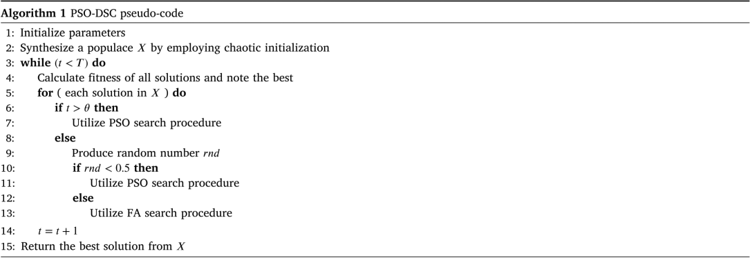

Close

Export to PPT

4 Experimental setup, analysis and discussion

The suggested methods are evaluated by employing real-world spot pricing data from Amazon EC2’s ’us-west’ area. The dataset covers huge Linux VMs. Inputs include ‘c38xlarge’,‘m44xlarge’, and ‘r38xlarge’, with the final price forecasting one step ahead. The dataset analysis starts from 24.03.2017. Due to the huge dataset sample size, a smaller sub-sample is used. Kaggle hosts the original dataset.¹ The available data is a 10-lag time-series. Data is split into training validation and evaluation subsets for investigation. An initial 70% (1200 samples) are allotted for training, 10% for validation and the remainder for evaluation.

Several metaheuristic optimizers are applied to the optimization of both LSTM and GRU networks in two separate experiments. A comparative analysis is carried out between the introduced modified algorithm and the original PSO (Kennedy and Eberhart, 1995). Additional algorithms included in the comparisons are “genetic algorithm” (Mirjalili and Mirjalili, 2019) (GA) and COLSHADE (Gurrola-Ramos et al., 2020) optimizes. Well-established swarm optimizes such as the “firefly algorithm” (Yang, 2009) (FA), “artificial bee colony” (Karaboga and Basturk, 2008) (ABC) and ”Harris hawk optimizes“ (Heidari et al., 2019) (HHO) are also included. The ”variable neighborhood search” (Mladenović and Hansen, 1997) (VNS) algorithm is also used in the comparative analysis. Each optimizer is given a population size of five and five iterations to enhance population quality. To accommodate for randomness, simulations are conducted over 30 times independently. To prevent over-training an early stopping criterion is used based on the equal to one-third of training epochs. Parameter ranges from both LSTM and GRU are optimized from a constrained including learning rate $[0,0001,0.01]$ , dropout $[0.05,0.2]$ , epochs $[10,30]$ , neurons per layer $[10,30]$ .

Evaluation of models involves standard regressing measures such as “root mean square error” (RMSE), “mean absolute error” (MAE), “mean square error” (MSE), and “coefficient of determination” ( $R^2$ ). The objective metric is MSE, and R ${}^2$ is the indicator function. An additional metric, the index of agreement (IoA), was used to evaluate synthesized models (Eq. (13)).

A flowchart of the proposed experimental framework describing dataset preparation, and the optimization process is provided in Fig. 1.

Close

Fig. 1

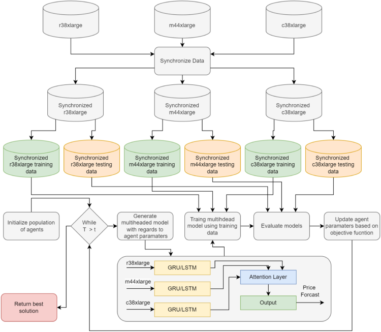
Introduced optimization framework flowchart.

Export to PPT

4.1

4.1 Simulation outcomes

4.1.1

4.1.1 Simulations with LSTM networks

The objective (MSE) function outputs for the best, worst mean, and median LSTM simulations are presented in Table 1, followed by comprehensive evaluations within the most promising models. The proposed optimizer demonstrates impressive outcomes, outperforming all competing metaheuristics demonstrating an MSE of $1.33E-06$ in the best-case execution. Furthermore, the proposed optimizer achieved the highest outcome for the median and mean cases demonstrating an objective function score of 1.48E−06 and 1.33E−06 respectively. The FA algorithm demonstrates adorable stability, with more stability evaluations shown in Fig. 2. As showcased in the stability diagrams, the introduced algorithm outperforms the original algorithm in all cases as well as competing metaheuristics demonstrating better results. While the stability is comparatively lower than some optimizers such as the original PSO, GA, and FA, the results attained by these optimizers are below even the worst results attained by the introduced optimizer.

Table 1 Outcomes for LSTM simulations.

Overall comparisons
Method	Best	Worst	Mean	Median	Std	Var
MHLSTM-PSO-DSC	1.33E−06	1.66E−06	1.48E−06	1.33E−06	1.67E−07	2.77E−14
MHLSTM-PSO	1.54E−06	1.64E−06	1.59E−06	1.59E−06	5.03E−08	2.53E−15
MHLSTM-GA	1.53E−06	1.62E−06	1.57E−06	1.53E−06	4.51E−08	2.04E−15
MHLSTM-VNS	1.71E−06	1.74E−06	1.72E−06	1.71E−06	1.44E−08	2.08E−16
MHLSTM-ABC	1.67E−06	1.78E−06	1.73E−06	1.78E−06	5.55E−08	3.08E−15
MHLSTM-FA	1.69E−06	1.70E−06	1.69E−06	1.70E−06	2.17E−09	4.71E−18
MHLSTM-HHO	1.41E−06	1.68E−06	1.53E−06	1.41E−06	1.35E−07	1.81E−14
MHLSTM-COLSHADE	1.67E−06	1.89E−06	1.79E−06	1.89E−06	1.07E−07	1.15E−14
Detailed Comparisons
Method	R${}^2$	MAE	MSE	RMSE	IoA
MHLSTM-PSO-DSC	0.191541	0.000908	1.33E−06	0.001152	0.531649
MHLSTM-PSO	0.061297	0.000990	1.54E−06	0.001241	0.510089
MHLSTM-GA	0.066289	0.001044	1.53E−06	0.001238	0.472012
MHLSTM-VNS	−0.043414	0.001118	1.71E−06	0.001308	0.142093
MHLSTM-ABC	−0.020013	0.001119	1.67E−06	0.001294	0.314240
MHLSTM-FA	−0.030752	0.001149	1.69E−06	0.001300	0.200151
MHLSTM-HHO	0.139422	0.000971	1.41E−06	0.001188	0.433447
MHLSTM-COLSHADE	−0.018482	0.001127	1.67E−06	0.001293	0.115080

Close

Fig. 2

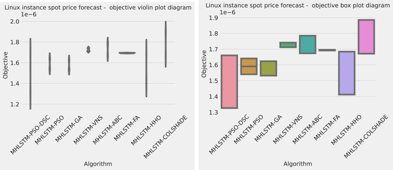
Objective function distribution plots for LSTM optimizations.

Export to PPT

4.1.2

4.1.2 Simulations with GRU networks

Outcomes in terms of objective (MSE) function for the best, worst mean and median GRU simulations followed by detailed comparisons between the best models are provided in Table 2. The introduced optimizer demonstrates impressive outcomes, outperforming all competing metaheuristics, producing an MSE of $1.16E-06$ in the best-case execution, and outperforming LSTM models as well. Furthermore, the introduced optimizer attained the best outcome for the worst, median, and mean cases demonstrating an objective function score of respectively. The highest rate of stability is showcased by the original PSO algorithm despite this optimizer not matching the performance of the modified algorithm. Further comparisons in terms of stability are provided in Fig. 3. As showcased in the stability diagrams, the introduced algorithm outperforms the original algorithm in all cases as well as competing metaheuristics demonstrating better results. While the stability is comparatively lower than some optimizers such as the original PSO, GA, and FA, the results attained by these optimizers are below even the worst results attained by the introduced optimizer. The best-performing model was optimized by the introduced modified metaheuristic and demonstrates the best outcomes across all metrics for the given challenge.

Further details on optimizer capabilities to balance exploration and exploitation while avoiding local minimum traps are provided in Fig. 4. The introduced optimizer manages to avoid a local trap in the third iteration of the optimization locating a more promising area of the search space by the 3rd iteration, suggesting that the introduced modifications help the modified algorithm locate more promising areas within the search space.

Table 2 Outcomes for each optimizer included in comparative analysis.

Overall Comparisons
Method	Best	Worst	Mean	Median	Std	Var
MHGRU-PSO-DSC	1.16E−06	1.23E−06	1.20E−06	1.23E−06	3.41E−08	1.16E−15
MHGRU-PSO	1.37E−06	1.38E−06	1.38E−06	1.37E−06	3.86E−09	1.49E−17
MHGRU-GA	1.64E−06	2.05E−06	1.90E−06	2.05E−06	1.97E−07	3.89E−14
MHGRU-VNS	1.32E−06	1.33E−06	1.32E−06	1.33E−06	5.86E−09	3.44E−17
MHGRU-ABC	1.41E−06	1.63E−06	1.52E−06	1.52E−06	1.09E−07	1.20E−14
MHGRU-FA	1.47E−06	1.48E−06	1.47E−06	1.47E−06	5.92E−09	3.51E−17
MHGRU-HHO	1.30E−06	1.62E−06	1.47E−06	1.62E−06	1.63E−07	2.65E−14
MHGRU-COLSHADE	1.69E−06	1.96E−06	1.81E−06	1.69E−06	1.32E−07	1.76E−14
Detailed Comparisons
Method	R${}^2$	MAE	MSE	RMSE	IoA
MHGRU-PSO-DSC	0.290191	0.000801	1.16E−06	0.001079	0.678492
MHGRU-PSO	0.162884	0.000985	1.37E−06	0.001172	0.389012
MHGRU-GA	0.000602	0.001105	1.64E−06	0.001281	0.056272
MHGRU-VNS	0.197970	0.000963	1.32E−06	0.001147	0.592289
MHGRU-ABC	0.139642	0.000987	1.41E−06	0.001188	0.435323
MHGRU-FA	0.107040	0.001065	1.47E−06	0.001210	0.435001
MHGRU-HHO	0.209853	0.000944	1.30E−06	0.001139	0.560155
MHGRU-COLSHADE	−0.030043	0.001084	1.69E−06	0.001300	0.179363

Close

Fig. 3

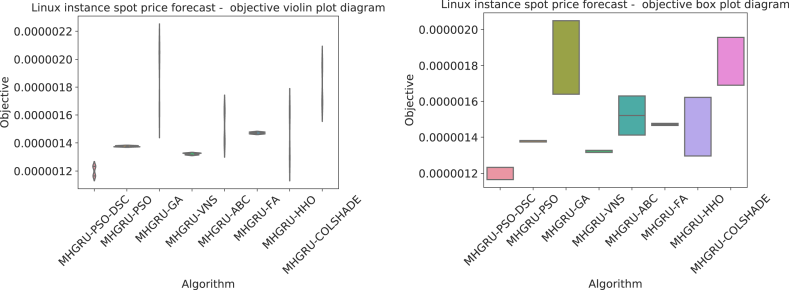
Objective function distribution plots for GRU optimizations.

Export to PPT

Parameter selections for the best GRU models as follows: a learning rate of 0.000194, dropout of 0.050000, 30 training epochs neurons in the first head 11, 30 in the second and 14 in the third heads. A total of 28 is utilized in the dense concatenation layer.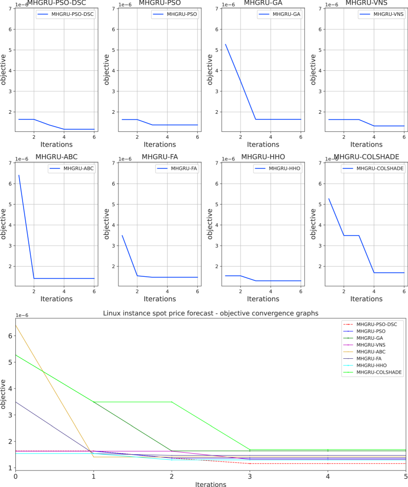

Close

Fig. 4

Convergence diagrams for GRU optimizations.

Export to PPT

4.4

4.4 Best-performing model interpretation

Understanding the factors that influence a model’s decisions is crucial. SHAP (Lundberg and Lee, 2017) is useful for obtaining insights. The best-constructed forecasting GRU model is subjected to SHAP interpretation. A high importance is given to r38xlarge samples 3 lags back followed by the same feature six months back. This is then followed by the m44xlrage one lag back. While their contribution is modest, the cumulative contributions contribute towards more accurate forecasting being made by the best-constructed model (see Fig. 5).

Close

Fig. 5

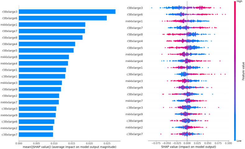
Best Performing GRU model SHAP interpretations.

Export to PPT

5 Conclusions

This study deals with the challenging and costly problem of cloud instance price forecasting. With more infrastructure relying on cloud services, a stable and predictable cost model will help companies supervise spending and optimize operations. Forecasting prices can help providers maintain consistency in billing clients. Multi-headed recurrent architecture is explored for LSTM and GRUs. Metaheuristic optimizers tune model parameters because network performance hinders architectural selection and training parameter sets. A modified version of the PSO optimizer enhances GRU and LSTM models, which forecast cloud instance pricing on a real-world dataset. The GRU models optimized by the new approach performed best with an MAE score of 0.000801. The proposed optimizer’s improvements enhance convergence rates, prevent premature stagnation and allow agents to find better search space solutions. The outcomes are analyzed statistically, and the best model is analyzed using explainable AI approaches to determine the features that boost forecasts.

High computation demands of optimization and model training limit the dataset size for analysis. Furthermore, high processing demands limit the number of optimizers in the comparative analysis. Scalability concerns when applying the proposed methodology to a larger dataset might increase forecasting model training demands. It is intended to explore and refine the forecasting method in the future. As more resources become available, other well-established optimizers will be compared to the introduced approach, and its uses will be examined.

CRediT authorship contribution statement

Mohamed Salb: Writing – review & editing, Validation, Software, Methodology. Luka Jovanovic: Writing – review & editing, Visualization, Validation, Supervision, Software, Methodology, Data curation. Ali Elsadai: Writing – review & editing, Validation, Resources, Methodology, Funding acquisition, Formal analysis. Nebojsa Bacanin: Writing – review & editing, Writing – original draft, Validation, Supervision, Methodology. Vladimir Simic: Writing – review & editing. Dragan Pamucar: Writing – review & editing. Miodrag Zivkovic: Writing – review & editing, Validation, Supervision.

References

- Deconstructing Amazon EC2 spot instance pricing. ACM Trans. Econ. Comput. (TEAC). 2013;1(3):1-20.
- [Google Scholar]
- Multi-swarm algorithm for extreme learning machine optimization. Sensors. 2022;22(11):4204.
- A novel fire algorithm approach for efficient feature selection with COVID-19 dataset. Microprocess. Microsyst.. 2023;98:104778
- Time series forecasting with multi-headed attention-based deep learning for residential energy consumption. Energies. 2020;13(18):4722.
- Cheng, R., Li, M., Tian, Y., Xiang, X., Zhang, X., Yang, S., Jin, Y., Yao, X., 2018. Benchmark Functions for the Cec’2018 Competition on Many-Objective Optimization. Technical Report.
- Putting analytics on the spot: or how to lower the cost for analytics. IEEE Internet Comput.. 2014;18(5):70-73.
- Kalman filtering for estimation and prediction servers with lower traffic loads for transferring high-level processes in cloud computing. Published by HCTL Int. J. Technol. Innov. Res. (ISSN: 2321-1814). 2017;23(1):10-20.
- Proposing new intelligence algorithm for suggesting better services to cloud users based on Kalman filtering. Published by J. Comput. Sci. Appl. (ISSN: 2328-7268). 2017;5(1):11-16.
- Involving Kalman filter technique for increasing the reliability and efficiency of cloud computing. In: Proceedings of the International Conference on Scientific Computing. The Steering Committee of The World Congress in Computer Science, Computer …; 2012. p. :1.
- Prediction and estimation of next demands of cloud users based on their comments in CRM and previous usages. In: 2018 International Conference on Communication, Computing and Internet of Things. IEEE; 2018. p. :81-86.
- Gate-variants of gated recurrent unit (GRU) neural networks. In: 2017 IEEE 60th International Midwest Symposium on Circuits and Systems. IEEE; 2017. p. :1597-1600.
- LSTM: A search space odyssey. IEEE Trans. Neural Netw. Learn. Syst.. 2016;28(10):2222-2232.
- COLSHADE for real-world single-objective constrained optimization problems. In: 2020 IEEE Congress on Evolutionary Computation. IEEE; 2020. p. :1-8.
- Service discovery mechanisms in cloud computing: a comprehensive and systematic literature review. Kybernetes. 2022;51(3):952-981.
- Machine learning applications in internet-of-drones: Systematic review, recent deployments, and open issues. ACM Comput. Surv.. 2023;55(12):1-45.
- Harris hawks optimization: Algorithm and applications. Future Gener. Comput. Syst.. 2019;97:849-872.
- Cloud-based non-destructive characterization. Non-Destruct. Mater. Charact. Methods 2024:727-765.
- A reliable method for data aggregation on the industrial internet of things using a hybrid optimization algorithm and density correlation degree. Cluster Comput. 2024:1-19.
- Tuning machine learning models using a group search firefly algorithm for credit card fraud detection. Mathematics. 2022;10(13):2272.
- Sine cosine algorithm with tangent search for neural networks dropout regularization. In: Data Intelligence and Cognitive Informatics: Proceedings of ICDICI 2022. Springer; 2022. p. :789-802.
- An emperor penguin optimizer application for medical diagnostics. In: 2022 IEEE Zooming Innovation in Consumer Technologies Conference. IEEE; 2022. p. :191-196.
- On the performance of artificial bee colony (ABC) algorithm. Appl. Soft Comput.. 2008;8(1):687-697.
- Particle swarm optimization. In: Proceedings of ICNN’95-International Conference on Neural Networks. Vol 4. IEEE; 1995. p. :1942-1948.
- A prescription of methodological guidelines for comparing bio-inspired optimization algorithms. Swarm Evol. Comput.. 2021;67:100973
- A unified approach to interpreting model predictions. In: Guyon I., Luxburg U.V., Bengio S., Wallach H., Fergus R., Vishwanathan S., Garnett R., eds. Advances in Neural Information Processing Systems 30. Curran Associates, Inc.; 2017. p. :4765-4774.
- The NIST definition of cloud computing. 2011.
- Proposing new method for clustering and optimizing energy consumption in WSN. Talent Dev. Excell.. 2020;12
- An approximate analysis of variance test for normality. J. Am. Stat. Assoc.. 1972;67(337):215-216.
- Dynamic price prediction for amazon spot instances. In: 2015 48th Hawaii International Conference on System Sciences. IEEE; 2015. p. :1513-1520.
- No free lunch theorems for optimization. IEEE Trans. Evol. Comput.. 1997;1(1):67-82.
- Firefly algorithms for multimodal optimization. In: Stochastic Algorithms: Foundations and Applications: 5th International Symposium, SAGA 2009, Sapporo, Japan, October 26–28, 2009. Proceedings 5. Springer; 2009. p. :169-178.
- Firefly algorithm. In: Swarm Intelligence Algorithms. CRC Press; 2020. p. :163-174.
- Best practice performance of COVID-19 in America continent with artificial intelligence. Spectr. Oper. Res.. 2024;1(1):1-12.
- [CrossRef] [Google Scholar]
- A framework for extensive content-based image retrieval system incorporating relevance feedback and query suggestion. Spectr. Oper. Res.. 2024;1(1):13-32.
- Feature selection using modified sine cosine algorithm with COVID-19 dataset. In: Evolutionary Computing and Mobile Sustainable Networks: Proceedings of ICECMSN 2021. Springer; 2022. p. :15-31.