Biresponse nonparametric regression model in principal component analysis with truncated spline estimator

1 Introduction

At this time, we have entered the era of big data on the number of samples, responses, and predictor variables. What concerns us here is that the larger the data, the greater the likelihood of assumptions for error correlation and multicollinearity in the predictors. One popular statistical approach to addressing this problem is principal component analysis (PCA). Several researchers who have studied PCA include Jolliffe and Cadima (2016) have developed PCA, which can reduce predictor variables through eigenvalues so that the components are mutually independent. The ability of PCA has been demonstrated by Bouwmans and Zahzah (2014) in image data analysis. Ghasemi et al. (2013) have classified the mineral composition of water samples, Vichi and Saporta (2009) have classified economic problems, and Hannachi et al. (2006) on climate issues. All of these PCA studies used a parametric approach that was limited to constructing the major components for a single response.

Another problem that can occur is that there are multicollinearity data that have an irregular pattern or do not follow a parametric pattern so that it is difficult to model it with the PCA parametric regression approach. Therefore, researchers developed nonparametric regression research, including Durand (1993) who has worked on instrumental variables with spline transformations. Wang et al. (2016) used PCA local polynomials and Shiokawa et al. (2018) with the PCA kernel. The use of another estimator by Lavado and Calapez (2011) have developed PCA with M Spline. For the spline estimator, there is a spline that contains a penalty function in its estimation criteria that can be used to overcome multicollinearity, namely spline smoothing by Lestari et al. (2010) and spline penalized by Islamiyati et al. (2020a). However, there is also another spline estimator that does not contain a penalty function, namely the truncated spline which cannot overcome the multicollinearity of the predictor. Therefore, in this article, we are developing a study on spline truncated PCA for two responses.

On a larger response dimension in nonparametric regression studies, Soo and Bates (1996) have developed a multi-response spline estimator using the Generalized Gauss-Newton algorithm. Wang, et al. (2000) have analyzed the bivariate data with the smoothing spline estimator. Furthermore, Chamidah et al. (2012) examined the use of local polynomial estimators in nonparametric regression. Zahra and Mhlawy (2013) made a numerical study on an exponential spline. Khan and Shahna (2019) used a quadratic spline. Tohari and Chamidah (2020) used a negative bi-response binomial regression with a linear local estimator. Furthermore, Islamiyati et al. (2018) developed a penalized spline estimator in the longitudinal biresponse case. However, all these studies have not considered the multicollinearity cases that can occur in large predictor data dimensions. They only consider the correlations that occur in responses that are overcome by weight in the estimation criteria, such as using weight in the variance–covariance matrix.

We demonstrated the capabilities of the method through simulation data and compared it with the parametric regression model approach, PCA, and the nonparametric spline regression model. Next, we applied it to real data, namely data on type 2 diabetes mellitus that we obtained from the Hasanuddin University Teaching Hospital. Islamiyati et al. (2020b) has examined the effect of treatment time on blood sugar through a longitudinal penalized spline. Islamiyati et al. (2020c) examined the pattern of changes in blood sugar based on the diet of diabetic patients through a biresponse approach Islamiyati et al. (2020c); Zahra and Mhlawy (2013). Furthermore, Islamiyati (2022) obtained several segments of changes in blood sugar based on lifestyle factors of diabetic patients. All of them indicate that the blood sugar fits the spline approach because there are changes at certain intervals.

2 Spline truncated function in the PCA

Given the pairs of observation data $\left(t_{i1},t_{i2},\dots t_{\mathit{ip}},y_{1.i},y_{2.i}\right)$ , the predictor variable t as many as p and the response variable y as many as two which follow the nonparametric pattern in $i=1,2,\dots ,n$ . If it is assumed that the predictor variables are strongly correlated, then multicollinearity occurs and must first be resolved. In a statistical approach, one method of handling multicollinearity is principal component analysis (PCA) which has been widely used in many applications. Jolliffe and Cadima (2016) explain that PCA reduces a group of predictor variables into a group of new variables as much as predictors called principal component. It is a linear combination of predictor variables in which the number of principal components formed is as many as predictors. The assumption is that the components are orthogonal so that they are not correlated and it is believed that the information provided does not overlap.

It is known that $\mathbf{\Sigma }$ is the variance matrix of the predictor variable $t_1,t_2,\dots ,t_p$ which is used as the basis for selecting the number of main components. If c is the main component, then the equation for each component can be stated as follows:

Eq. (1) can also be expressed in vector form, namely: $${\underset{\sim }{c}}_1=\mathit{T}{\underset{\sim }{\gamma }}_1,{\underset{\sim }{c}}_2=\mathit{T}{\underset{\sim }{\gamma }}_2,\dots ,{\underset{\sim }{c}}_p=\mathit{T}{\underset{\sim }{\gamma }}_p$$ where $c_1,c_2,\dots ,c_p$ is called the principal component 1, 2,…, p and each has a variance of ${\lambda }_1,{\lambda }_2,\dots ,{\lambda }_p$ , T is the predictor matrix and $\underset{\sim }{\gamma }$ is the principal component coefficient vector. The order of the main components is taken based on the large variety so that the largest variance is in the 1st component and the smallest variance is in the p-component with ${\underset{\sim }{\gamma }}_1={\left({\gamma }_{1.1},{\gamma }_{1.2},\dots ,{\gamma }_{1.p}\right)}^T$ and ${\underset{\sim }{\gamma }}_1^T{\underset{\sim }{\gamma }}_1=1$ . Suppose ${\lambda }_1⩾{\lambda }_2⩾\cdots ⩾{\lambda }_p$ is the characteristic root corresponding to the feature vector ${\underset{\sim }{\gamma }}_1,{\underset{\sim }{\gamma }}_2,\dots ,{\underset{\sim }{\gamma }}_p$ of the matrix $\mathbf{\Sigma }$ and ${\underset{\sim }{\gamma }}_1^T{\underset{\sim }{\gamma }}_1=1$ for $j=1,2,\dots ,p$ , then ${\underset{\sim }{c}}_1=\mathit{T}{\underset{\sim }{\gamma }}_1,{\underset{\sim }{c}}_2=\mathit{T}{\underset{\sim }{\gamma }}_2,\dots ,{\underset{\sim }{c}}_p=\mathit{T}{\underset{\sim }{\gamma }}_p$ is the 1st, 2nd,…, p^th principal component of t. For data applications, the number of principal components is selected based on the cumulative variance described by the components.

In many multivariate studies, the principal component problem only comes to Eq. (1), which describes the principal components that are formed based on their total variety. However, the problem is different when our data is nonparametric. To model the data, the principal components obtained in Eq. (1) are then connected to the predictors through an estimator function in nonparametric regression, namely the truncated spline.

If the principal component selected is m from p component and is symbolized by $c_j,j=1,2,\dots ,m,\dots ,p$ for $m⩽p$ , then the principal component function of the truncated spline based on the predictor can be stated as follows:

The function of each predictor $\left(f_j\left(t_1\right),f_j\left(t_2\right),\dots ,f_j\left(t_p\right)\right)$ in (2) is a vector of the spline function of unknown shape for $j=1,2,\dots ,m$ . It is estimated with a truncated spline in the order q and the point of knots K. The spline function in each predictor for each j^th component can be described as follows:

Eq. (3) can be expressed in vector form, which is as follows: $$f_j\left(t_1\right)+f_j\left(t_2\right)+\dots +f_j\left(t_p\right)={\mathit{X}}_j{\underset{\sim }{\beta }}_j$$ where X is the predictor matrix containing the knots point and ${\underset{\sim }{\beta }}_j={\left({\underset{\sim }{\beta }}_1,{\underset{\sim }{\beta }}_2,\dots ,{\underset{\sim }{\beta }}_p\right)}^T$ is the feature vector for each predictor.

Furthermore, the spline function of the first principal component can be stated as follows: $${\underset{\sim }{c}}_1={\mathit{X}}_1{\underset{\sim }{\beta }}_1+{\underset{\sim }{\xi }}_1$$ where ${\underset{\sim }{\beta }}_1={\left({\beta }_{1.1},{\beta }_{1.2},\dots ,{\beta }_{1.p}\right)}^T$ .

Furthermore, the spline function of the second main component, up to p, can be stated as follows: $${\underset{\sim }{c}}_2={\mathit{X}}_2{\underset{\sim }{\beta }}_2+{\underset{\sim }{\xi }}_2,\dots ,{\underset{\sim }{c}}_p={\mathit{X}}_p{\underset{\sim }{\beta }}_p+{\underset{\sim }{\xi }}_p$$

3 Biresponse nonparametric regression model with spline PCA

The biresponse nonparametric regression model on PCA is a nonparametric regression model that contains two response variables (y_r) with $r=1,2$ and several main component variables (c_j). Suppose that the number of main components selected is m, then the observation data pair $\left(c_{i1},c_{i2},\dots c_{\mathit{im}},y_{1.i},y_{2.i}\right)$ , with $i=1,2,\dots ,n$ , satisfies the biresponse nonparametric regression model as follows:

The model in (4) can be stated as:

Eq. (5) can also be written in matrix form, namely:

Furthermore, the Eq. (7) as a biresponse nonparametric regression model in PCA spline, it was estimated using weighted least square (WLS). The WLS estimator symbolized by P is as follows: $$\text{P}={\underset{\sim }{\epsilon }}^T{\widehat{\mathit{\theta }}}^{-1}\underset{\sim }{\epsilon }$$

Further obtained:

Based on the estimation results of the regression parameters in (8), we get an estimate of the biresponse nonparametric regression model on PCA through a truncated spline estimator as in Eq. (9).

4 Simulation data

We make different experimental functions on the predictors, namely $f\left(t_{i1}\right)$ is in the form of polynomial while $f\left(t_{i2}\right)$ and $f\left(t_{i3}\right)$ is in the form of trigonometry. The number of subjects tested was n = 10, 30, 50, 100, 150 with correlation between predictors between 0.7 and 0.8. In this study, we choose a positive correlation because it is related to the condition variable to the real data. Simulations are being performed on a single response to demonstrate the ability of the PCA spline to model multicollinearity nonparametric data. The nonparametric regression model follows $y_i=f\left(t_{i1},t_{i2},t_{i3}\right)+{\epsilon }_i$ with $i=1,2,\dots ,n$ . The functions of the 1st predictor, 2nd predictor, and 3rd predictor are indicated by $f\left(t_{i1}\right)=0.6t_i^2+2t_{i1}+3$ , $f\left(t_{i2}\right)=3\times \text{sin}\left(2\pi t_{i2}\right)$ , and $f\left(t_{i3}\right)=5+2sin\left(\pi t_{i3}\right)$ .

In this section, we present a data plot for a sample size of n = 150 as shown in Fig. 1 for the 1st, 2nd, and 3rd predictors, respectively. The results of the correlation test between the predictors showed that there was multicollinearity in the data where there was a strong correlation between t₁ and t₂ of 0.86, t₁ and t₃ of 0.82, t₂ and t₃ of 0.71. In this article, the predictors are reduced to independent components via PCA with 3 principal components that correspond to the number of predictors. Based on the value of the cumulative proportion which can also be seen through the scree plot in Fig. 2, we take two principal components to be analyzed because the proportion of variance that can be explained has reached 97%. Furthermore, the predictor variables entered into each component are shown through the loading factor. The first component contains the three predictors, namely t₁, t₂, and t₃, while the second component contains only two predictors, namely t₂ and t₃. This indicates that the simulation data can be made into two independent components with each influencing predictor. There are two different conditions in the data, one is that there is a group of data that is influenced by all the predictors and there is another group that is only affected by two predictors. However, in the data, it is not only multicollinearity that occurs, but the data also has plots that do not follow a parametric pattern. The use of PCA alone has not been able to solve the problems that occur in the data. Therefore, in this study, we estimated the principal component based on the predictor through the truncated spline. Through the loading factor in PCA, it is shown the factors that significantly influence each main component. Significant predictors were then estimated from PC values through the nonparametric regression model of spline truncated PCA.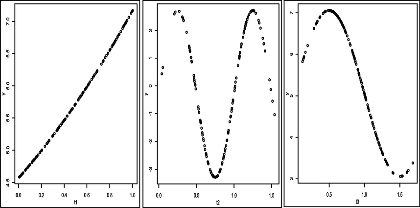

Close

Fig. 1

Plot of data between predictors and responses.

Export to PPT

Close

Fig. 2

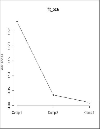
Scree plot of simulation data.

Export to PPT

Fig. 3a shows the first component contains the significant predictors, t₁, t₂ and t₃ and shows an ascending linear pattern. The second component contains the t₂ and t₃ predictors shown in Fig. 3b. Furthermore, the two main components were modeled based on significant predictors through truncated spline PCA. We model it using knot points of 1 to 11 knots. Based on the truncated spline PCA, we obtain a spline regression curve with several optimal knot points. There is a different regression curve for each selected knot point, both for the first and second components. Therefore, we need to select the optimal knot point for each major component through the minimum GCV and MSE values as in Table 1 which corresponds to the knot points in Table 2. The minimum GCV and MSE values obtained at c₁ for t₁, t₂, and t₃ are 11, 8 and 10 knots, respectively. The minimum GCV and MSE values at c₂ for t₂ and t₃ is 11 knots. These results indicate that the minimum GCV and MSE values is obtained at different knot points for each component. Where the knot point is the starting point for a pattern change in the main component.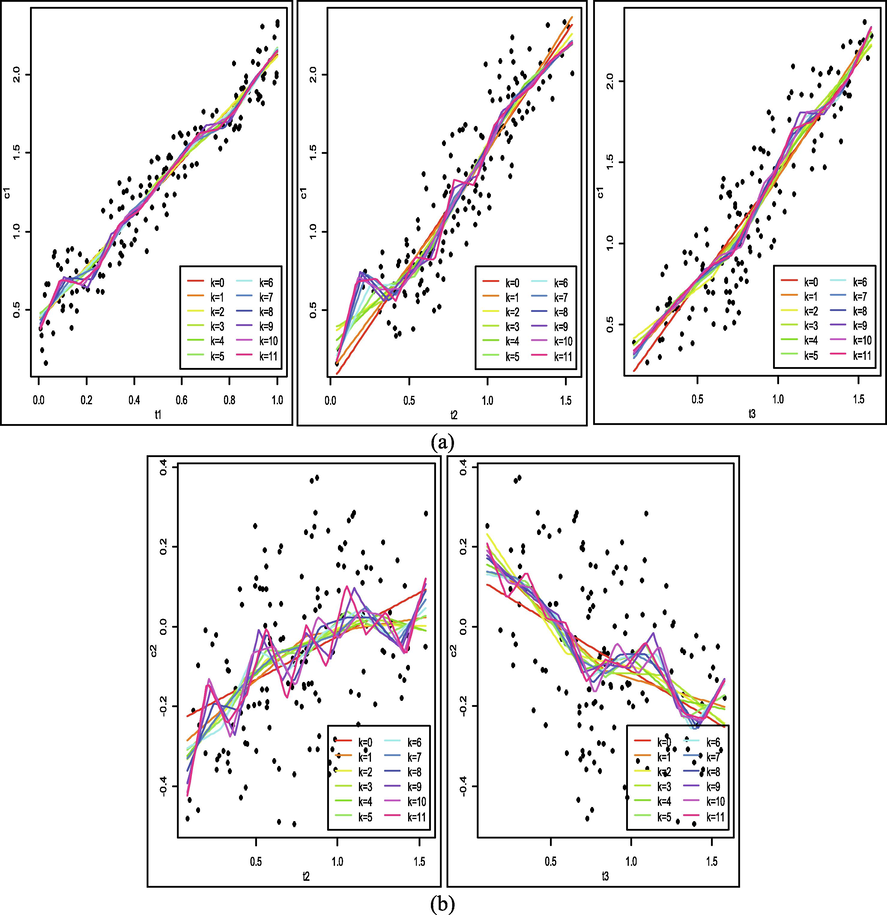

Close

Fig. 3

The estimation results of the PCA spline regression curve at several knots for (a) the first component and (b) the second component.

Export to PPT

Furthermore, Fig. 4 shows a box plot of the MSE value which aims to compare the estimated results of the PCA spline with the multiple linear regression model and PCA. The use of the MSE value in the plot is because the model we used as a comparison with the estimated results of the PCA spline is a parametric model. The results in Fig. 4 shows that the PCA spline provides a much smaller MSE value compared to the parametric linear regression and PCA models. Therefore, the Spline PCA nonparametric regression model is very suitable to be used to model data between predictors with responses that do not follow a parametric pattern and correlated variables.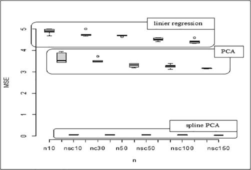

Close

Fig. 4

Boxplot MSE of linear regression, PCA and PCA spline.

Export to PPT

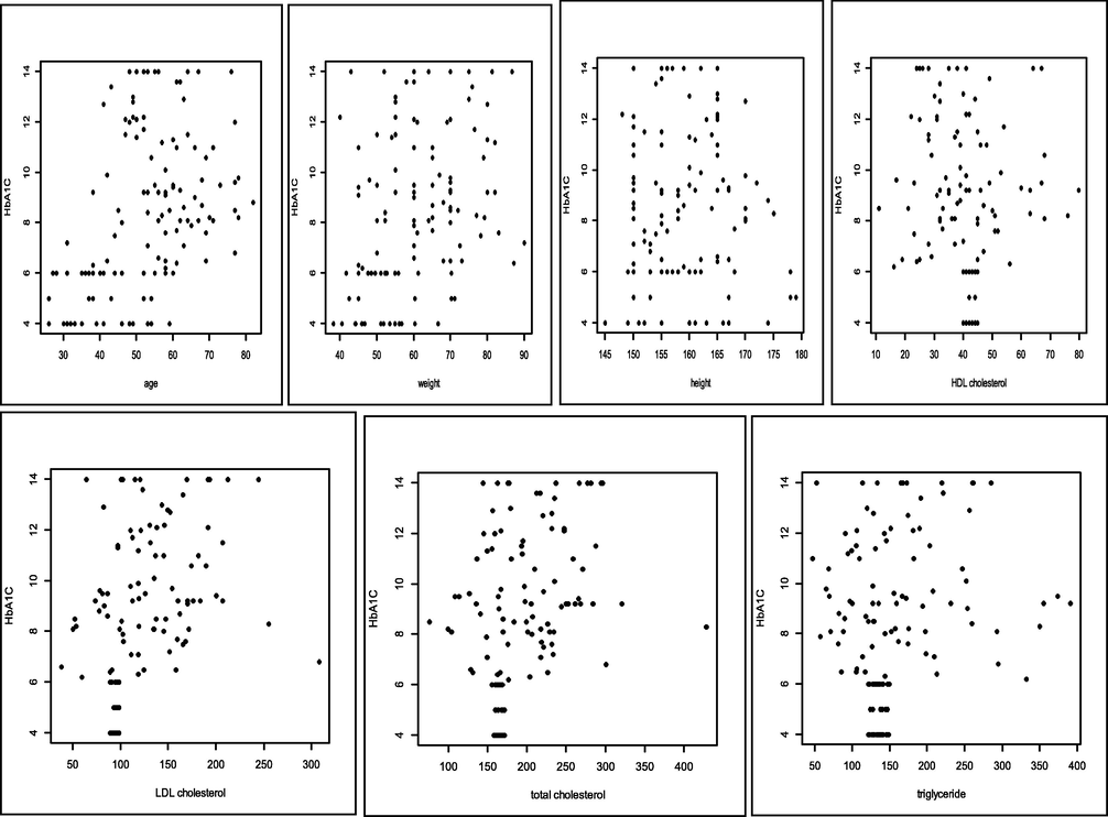
5 Application on type 2 diabetes mellitus data

The ability of the PCA spline method to be more accurate in the simulation data in the previous section has provided assurance that this method can be applied to diabetes data. The variables studied were fasting blood sugar and HbA1C as the first and second responses, respectively. The factors of age, weight, height, HDL cholesterol, LDL cholesterol, total cholesterol, and triglycerides were the first, second, third, fourth, fifth, sixth, and seventh predictors, respectively. Data plots of fasting blood sugar levels are shown in Fig. 5 and HbA1C in Fig. 6. All figures show that the data plots between fasting blood sugar factors and HbA1C with LDL cholesterol, HDL cholesterol, total cholesterol, and triglyceride factors do not show a parametric plot. Therefore, we use a truncated spline as one of the estimators for non-parametric patterned data. This estimator is able to explain some pattern segmentation that occurs in the data through knot points. The patient's blood sugar is always changing in a fast time can be interpreted well by spline truncated through the knot point. Next, the correlation $r_{y_1.y_2}=0.780$ , $r_{t_2.t_3}=0.856$ and $r_{t_3.t_4}=0.586$ . This shows a correlation between responses and multicollinearity in the predictor variables. To overcome these two types of correlation, we used a PCA biresponse model with a truncated spline estimator.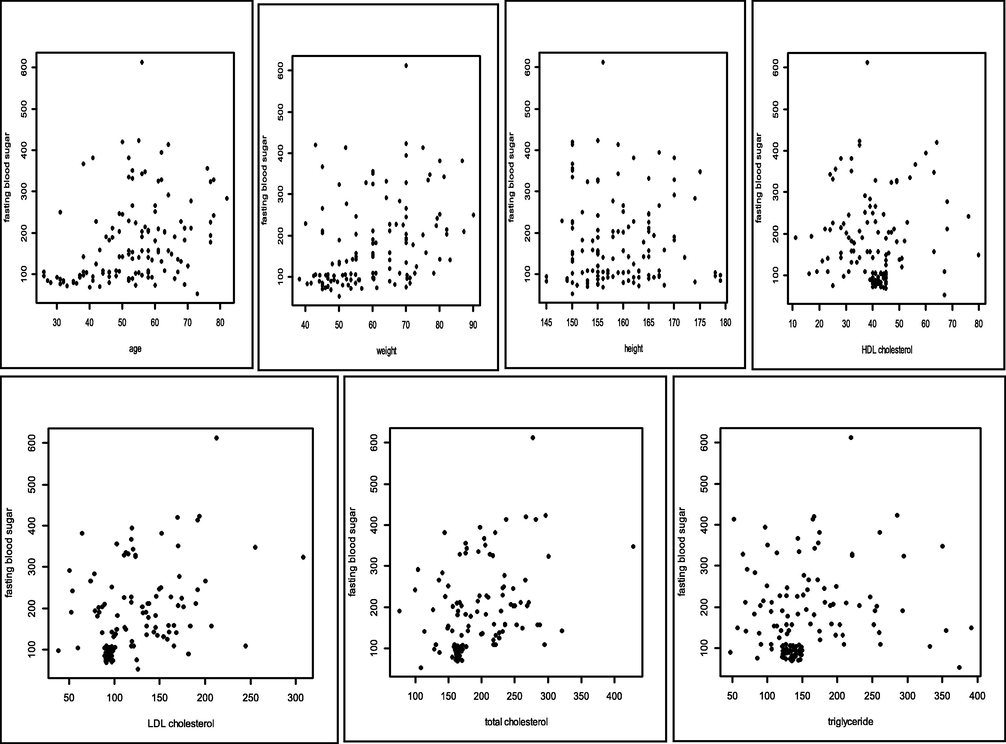

Close

Fig. 5

The plot of fasting blood sugar (y₁) based on predictors.

Export to PPT

Close

Fig. 6

The plot of HbA1C (y₂) data based on predictors.

Export to PPT

Based on the Scree plot, we can take two main components of the seven main components, because it can explain the variance of 85.7%. Furthermore, we found that the significant predictor variables in the first and second components were the same, namely the variables LDL cholesterol, total cholesterol and triglycerides. These results indicate that the two groups of diabetic patients can be modeled and we only need to consider three factors from the seven factors studied, namely LDL cholesterol, total cholesterol, and triglycerides. From the value of the principal component that corresponds to the predictor, we can model the main component through the spline function truncated with a certain knot point.

The estimation results of the PCA spline regression curve between the first and second components with predictors are shown in Fig. 7. Based on Fig. 7a and b, the spline curve estimation of each component looks different from one another. In the cholesterol factor, namely LDL and total cholesterol, there is an upward trend in the first and second components, but the increase is different from one another. For triglyceride factors, there is an uptrend in the first component and a downtrend in the second component. The trend is indicated by optimal knot points where the points are selected based on the GCV value. In this data, we get 3 knot points which give the minimum GCV value, namely for LDL cholesterol factors are 105.5, 173, and 240.5, for total cholesterol factors are 164, 252, 340, and for triglyceride factors are 133, 219, 305.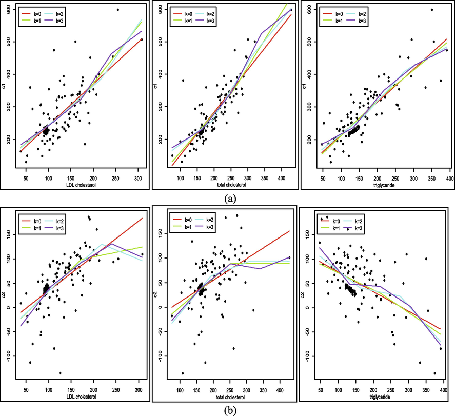

Close

Fig. 7

The estimation results of the truncated spline curve are based on the factors of LDL cholesterol, total cholesterol, and triglycerides on (a) the first component and (b) the second component.

Export to PPT

The spline equation is truncated on each component corresponding to the knot point are as follows:

Eq. (10) corresponds to Fig. 8 which shows the estimation results of the spline truncated curve for each principal component.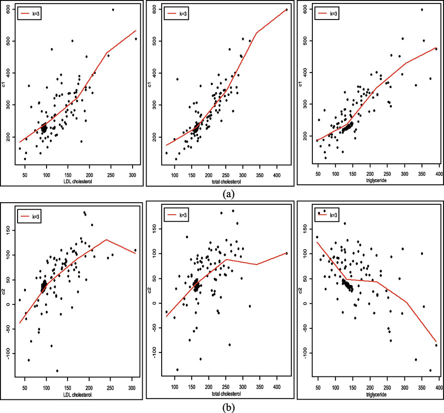

Close

Fig. 8

The estimation results of the spline truncated PCA curve for biresponse to (a) the fasting blood sugar factor and (b) the HbA1C factor.

Export to PPT

Furthermore, the biresponse PCA spline regression model obtained between the response and the main components of the diabetes data is as follows: $$\begin{array}{c}{y}_1=-37.905+0.184c_1+0.445c_2\\ y_2=1.885+0.005c_1+0.016c_2\end{array}$$

Based on the equation of the principal components in (10), the PCA biresponse spline regression model can be expressed as follows:

The results of the analysis of the biresponse PCA spline model showed a pattern of changes in fasting blood sugar and HbA1C levels, which were mostly influenced by LDL cholesterol, total cholesterol, and triglycerides. In the first component, fasting blood sugar and HbA1C tend to rise along with the increase in cholesterol and triglycerides. However, the increment varies at certain value intervals. Furthermore, for the second component, fasting blood sugar and HbA1C increased and decreased based on the patient's cholesterol and triglyceride levels in certain intervals. This shows that through spline truncated PCA biresponse, we can identify two conditions that can occur in patients with type 2 diabetes mellitus.

6 Conclusion

A bi-response truncated PCA spline model was developed for data containing multi-dimensional variables in which responses are correlated as well as predictors. The multicollinearity problem in predictors was solved by using PCA spline. The principal component that is formed is modeled with a predictor through a truncated spline estimator which considers the knot point. The ability of the method has been demonstrated through simulation data and MSE values were obtained that were smaller than the parametric regression and PCA approaches as shown in Fig. 4. This method is also applied to data on type 2 diabetes mellitus patients. Based on the results of the analysis of the biresponse spline PCA model, it was found that there were two main components which indicated that there were two different groups of type 2 diabetes mellitus patients. The two principal components are equally affected by LDL cholesterol, total cholesterol and triglycerides. What distinguishes these components is the pattern of changes in fasting blood sugar and HbA1C based on these three factors. The pattern can be seen in Fig. 8, and then modeled as in Eq. (10). The condition of the type 2 diabetes mellitus patients described in this article shows that the important factors that the patient should pay attention to are the regulation of LDL cholesterol, total cholesterol, and triglycerides. The shape of their influence on the patient is described in terms of two components. Also, the effect of these three factors shows that there are several patterns of change at certain intervals corresponding to the knot point. This result is one of the advantages of this method that cannot be explained through a parametric approach.

This research is sponsored by Deputy of Research and Development Strengthening, Ministry of Research and Technology/National Agency for Research and Innovation, Republic of Indonesia for the Basic Research, and will continue to be developed on both theory and data applications. There is an obligation for us to publish our research results as a form of review of the development of pre-existing methods. For that matter, no potential conflict will occur associated with this article, neither to funding nor to all authors.

References

- Robust PCA via principal component pursuit: a review fora comparative evaluation in video surveillance. Comput. Vis. Image Underst.. 2014;122:22-34.
- [Google Scholar]
- Designing of child growth chart based on multi response local polynomial modeling. J. Math. Stat.. 2012;8(3):342-347.
- Generalized principal component analysis with respect to instrumental variables via univariate spline transformation. Comput. Stat. Data An.. 1993;16(4):423-440.
- Linear and nonlinear multivariate classification of Iranian bottled mineral waters according to their elemental content determined by ICP-OES. J. Sci. Islam. Repub. Iran. 2013;24(1):15-22.
- In search of simple structures in climate: simplifying EOFs. Int. J. Climatol.. 2006;26(1):7-28.
- Estimation of covariance matrix on bi-response longitudinal data analysis with penalized spline regression. J. Phys.: Conf. Ser.. 2018;979(012093):1-8.
- Use of two smoothing parameters in penalized spline estimator for bi-variate predictor non-parametric regression model. J. Sci. Islam. Repub. Iran.. 2020;31(2):175-183.
- Changes in blood glucose 2 hours after meals in Type 2 diabetes patients based on length of treatment at Hasanuddin University Hospital, Indonesia. Rawal Medical J.. 2020;45(1):31-34.
- Penalized spline estimator with multi smoothing parameters in biresponse multipredictor regression model for longitudinal data. Songklanakarin J. Sci. Technol.. 2020;42(4):897-909.
- Islamiyati, A. 2022. Spline longitudinal multi-response model for the detection of lifestyle-based changes in blood glucose of diabetic patients. Curr. Diabetes Rev. E-pub Ahead of Print, Published on: 14 January, 2022.
- Principal component analysis: a review and recent developments. Phil. Trans. R. Soc. A.. 2016;374(2065):20150202.
- [CrossRef] [Google Scholar]
- Non-polynomial quadratic spline method for solving fourth order singularly perturbed boundary value problems. J. King Saud Univ. Sci.. 2019;31(4):479-484.
- Principal components analysis with spline optimal transformations for continuous data. IAENG Int. J. Appl. Math.. 2011;41(4):367-375.
- Spline smoothing for multi-response nonparametric regression model in case of heteroscedasticity of variance. J. Math. Stat.. 2010;8(3):377-384.
- Application of kernel principal component analysis and computational machine learning to exploration of metabolites strongly associated with diet. Sci. Rep.. 2018;8
- Modelling of HIV and AIDS cases in Indonesia using bi-response negative binomial regression approach based on local linear estimator. Ann. Biol. 2020;36(2):215-219.
- Clustering and disjoint principal component analysis. Comput. Stat. Data An.. 2009;53(8):3194-3208.
- A robust polynomial principal component analysis for seismic noise attenuation. J. Geophys. Eng.. 2016;13(6):1002-1009.
- Spline smoothing for bivariate data with application to association between hormones. Stat. Sin.. 2000;10:377-397.
- Numerical solution of two-parameter singularly perturbed boundary value problems via eksponential spline. J. King Saud Univ. Sci.. 2013;25(3):201-208.