

Translate this page into:
An inertial conjugate gradient projection method for large-scale nonlinear equations and its application in the image restoration problems
⁎Corresponding author. lujunwei2024@126.com (Chunzhao Liang),
-
Received: ,
Accepted: ,
This article was originally published by Elsevier and was migrated to Scientific Scholar after the change of Publisher.
Abstract
Based on the acceleration effect of the inertial extrapolation technique on the convergence of iterative sequences, the number of algorithms incorporating this technique has gradually increased in recent years. Currently, there is a relative paucity of studies focusing on the Polak-Ribière-Polyak (PRP) conjugate gradient algorithm that integrate the inertial extrapolation technique. In this article, we introduce an inertial three-term PRP conjugate gradient projection method by incorporating an inertial extrapolation step into the three-term PRP algorithm, where the search direction exhibits sufficient descent and trust region characteristics. The search rule employs a derivative-free technique. Under suitable hypotheses, the proposed algorithm demonstrates global convergence. Numerical results indicate the superiority and competitiveness of this innovative method. Furthermore, its effectiveness in addressing image restoration problems underscores the practicality of this algorithm.
Keywords
Monotone equations
Inertial extrapolation technique
Three-term PRP method
Global convergence

1 Introduction
Many practical problems can be approximated using the following model:
As a category of optimization problems, system (1.1) is not only extensively employed in the field of mathematics but also closely linked to real-world production and life. For instance, notable nonlinear fracture problems (Gregory et al., 1985) mathematics, chemical equilibrium issues (Meintjes and Morgan, 1987) that significantly influence industrial production, and image recovery challenges in the domain of compressed sensing (Xiao et al., 2011) can all be transformed into system (1.1) for resolution.
In recent decades, Various numerical iterative methods have been proposed to solve system (1.1). Notably, the incorporation of projection techniques (Solodov and Svaiter, 1999) has significantly enhanced the running speed of many iterative algorithms. These projection algorithms are categorized into two types: derivative-based algorithms and derivative-free algorithms. The former includes Newton-type method (Solodov and Svaiter, 1999; Zhou and Toh, 2005), quasi-Newton method (Zhou and Li, 2007, 2008; Chen et al., 2014), semi-smooth Newton method (Xiao et al., 2018) and trust region algorithm (Qi et al., 2004; Ulbrich, 2001). While these algorithms offer a rapid convergence rate as a primary advantage, the necessity of computing and storing the Jacobian or its approximate matrices poses challenges in solving large-scale equations, potentially reducing their efficiency and increasing computational time in practical applications. Consequently, the second category of methods, which does not require the computation and storage of Jacobian or its approximate matrices, has been developed to address these issues and ultimately enhance computational speed. The conjugate gradient (CG) method is a prominent example. Following the introduction of projection technology, Liu and Feng (2019) proposed a derivative-free projection method (DFPM) combined with the (PDY) method for convex constraint problems, demonstrating its Q-linear convergence. Subsequently, Sabi’U et al. (2020) introduced a new hybrid method that integrates the Fréchet-Robinson (FR) method and the PRP method with the projection strategy for monotone nonlinear equations, achieving a convergence rate significantly faster than that of the three-term PRP algorithm. For the same problems, Abubakar et al. (2021) modified a memoryless symmetric rank-one (SR1) update to develop two new algorithms, asserting their robustness. Afterward, numerous derivative-free projection methods has been proposed subsequently (Sabi’u et al., 2020; Koorapetse et al., 2021; Yin et al., 2021b,a; Sabi’u et al., 2024).
Many scholars aspire to enhance the convergence speed of iterative algorithms, leading to numerous attempts in this area (Chen et al., 2013; Iiduka, 2012; Jolaoso et al., 2021; Abubakar et al., 2020a,b, 2019). Recently, an inertial extrapolation technique has been proposed that can effectively accelerate the iteration process (Alvarez, 2004; Alvarez and Attouch, 2001). This technique, derived from the “heavy ball” method (Polyak, 1964), plays a importance role in improving the overall convergence rate of the algorithm.
Based on the acceleration effect of the inertial extrapolation technique on the convergence of iterative sequences, the number of algorithms incorporating this technique has gradually increased. For instance, this technique has been utilized to enhance various existing splitting methods (Chen et al., 2015; Pock and Sabach, 2016) and projection methods. A series of inertial DFPMs (Jian et al., 2022) have been proposed to address pseudo-monotone equations. In the field of compressed sensing, Ma et al. (2023) improved an inertial three-term CG projection method. Additionally, for convex constrained problems, an inertial Dai-Liao CG method has been proposed, which avoids the direction of maximum magnification (Sabi’U and Sirisubtawee, 2024).
Motivated by the derivative-free search strategy and the three-term PRP CG method in Yuan and Zhang (2015), we have incorporated an extrapolation strategy (Ibrahim et al., 2021) to develop the inertial three-term PRP CG projection algorithm, referred to as the ITTPRP algorithm. Under suitable conditions, we demonstrate that this new algorithm exhibits global convergence. Ultimately, a series of numerical results validate the superiority of the proposed algorithm.
The chapters of this article are organized as follows: In Section 2, we will present the ITTPRP algorithm. Section 3 provides a proof of convergence for the ITTPRP method. In Section 4, we will display results that validate the effectiveness of the ITTPRP method. Finally, Section 5 offers conclusions.
2 The algorithm
With the purpose of showing our algorithm, here is the general statement of the concept of projection operator
, which represents a mapping from
to
a nonempty closed convex set:
represents Euclidean norm, which has a character, ie, for any
,
The following are the detailed steps of the algorithm.
Algorithm 1 ITTPRP
Step 0.Input , and , Let .
Step 1.If
, then terminate. Else select an inertial extrapolation steplength
Step 2.If , then terminate. Else find the search direction by where .
Step 3.Find
, the steplength
such that
Step 4.If , terminate, and let . Else, calculate the next iterate by where
Step 5.Let . Back to step 1.
For all , it can be observed from Eq. (2.2) that . This implies that
If
and
are calculated by Algorithm ITTPRP, then
satisfies the characteristic of sufficient descent :
By the definition of
in Algorithm 1, it is easy to conclude that
for all
. If
or
, we have
. For
and
, we can deduce that
3 Global convergence
This section will provide a proof of convergence for the ITTPRP method. Some necessary hypotheses and lemmas are as follows.
(i) The solution set contains at least one valid solution, indicating that the solution set is non-empty.
(ii) The mapping is Lipschitz continuous, which means there is a positive number , for any ,
Assume Hypothesis is always valid, sequences and are formed by the ITTPRP algorithm, then for all , there is a nonnegative satisfying inequality (2.3).
By using reduction to absurdity, we can obtain the following result: Suppose there exists an integer greater than 0, which makes all nonnegative integers fail to satisfy (2.3). Therefore, for all , the subsequent inequality is always valid: Consider is continuous and , as , it satisfies that which contradicts with (2.4). Thus the proof is concluded.
Lemma 3.2 Auslender et al., 1999
Suppose and be nonnegative number sequences, then they satisfy the subsequent inequality: where , then exists.
Let hypothesis hold, and sequences , and are successively outputted by Algorithm 1. Assume that represents a solution to problem (1.1) with , which satisfies Moreover, the sequence is bounded and
Through the monotonicity of the mapping
, we can infer
If Hypothesis is always valid, we can deduce the following conclusions from Lemma 3.3.
(i) The is bounded.
(ii) .
(iii) The sequences , , and are all bounded.
(i) From Hypothesis A(ii) and (3.4), we have
(ii) By the concept of
and (3.7), having
, What is more, from Remark 2.1, considering that
, we can infer that
Thus,
If Hypothesis A is always valid. Let , and are generated by ITTPRP, and belongs to . Then, the convergence of , and to the same solution of problem (1.1) is ensured.
The proof will be divided into two parts.
Part I. We should exhibit that
. We will demonstrate this by reduction to absurdity, starting with the assumption that
Hence, there is a constant
satisfying
Part II. We show that , , and all converge to the same solution of problem (1.1). Since is bounded, is a continuous mapping, and the previous part has already established that . Based on these, we assume which indicates . Based on the first relation in (3.10) and Remark 3.1(ii), we can obtain is a convergence point of , implying there is an infinite set satisfying . Setting in Remark 3.1(ii), we have So, converges to . Based on Remark 3.1(ii), we can infer that both and also converge to . This proof is concluded.
4 Numerical results and discussions
Numerical experiments will be conducted in two modules. The first module involves solving nonlinear equations, while the second module focuses on an image restoration application.
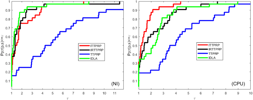
Performance profiles on NI and CPU.
4.1 Nonlinear equations
We conduct tests on nonlinear equations in this module. The problems to be tested and their corresponding initial points can be found in Yuan and Zhang (2015). For experimentation, we utilize the eight problems listed in Table 1, maintaining the same initial points as those in Yuan and Zhang (2015).
To demonstrate the superiority of the ITTPRP algorithm, We compared it to the IDLA algorithm (Sabi’U and Sirisubtawee, 2024), the TTPRP algorithm (Yuan and Zhang, 2015), and the inertial-relaxed TTPRP method which differs from ITTPRP by maintaining and introducing a relaxation factor in the projection step. Detailed information regarding the inertial-relaxed technique can be found in Yin et al. (2023). In this article, we refer to the inertial-relaxed TTPRP method as the IRTTPRP method.
The following were used for experimental comparison:
NO
Test problem
1
Exponential function
2
Trigonometric function
3
Logarithmic function
4
Broyden tridiagonal function
5
Trigexp function
6
Strictly convex function
7
Extended Freudentein and Roth function
8
Discrete boundary value problem
Dimensions: 5000, 10,000, 50,000, 100,000.
Parameters: We select and for ITTPRP. Furthermore, we set the relaxation factor for IRTTPRP and other parameters are consistent with ITTPRP. For TTPRP and IDLA, all parameters are cited from Yuan and Zhang (2015) and Sabi’U and Sirisubtawee (2024), respectively.
Stopping condition: The operations are terminated when any of the subsequent criteria is met: (i) , (ii) , (iii) , (iv) .
Implementation software: All experiments are operated in MATLAB R2020a on a 64-bit Lenovo laptop with lntel(R) Core(TM) i5-7200U CPU (2.70 GHz), 8.00 GB RAM and Windows 10.
The results from these methods are presented in Tables 2–5, where NO denotes the problem number, DIM indicates the dimension of the variable , IN represents the number of iterations, CPU signifies the running time in seconds, and GN refers the norm of the objective function. As illustrated in Fig. 1, ITTPRP, IRTTPRP, and IDLA significantly outperform TTPRP for nonlinear equations, suggesting that both inertial and inertial-relaxed techniques can enhance the convergence of the algorithm. Furthermore, the numerical results regarding NI and CPU demonstrate that the ITTPRP method outperforms both the IDLA and IRTTPR methods.
4.2 Image restoration problems
The objective of this part is to restore images that have been compromised by salt-and-pepper noise to their original state. The operating conditions and parameters remain consistent with those outlined in the previous section. The termination condition is or . For the experiments, we selected the images Peppers , ColoredChips and ColorChecker as subjects. To facilitate a comparison with ITTPRP, we also implemented IDLA, IRTTPRP, and TTPRP in our experiments. In this study, we employed the Peak Signal-to-Noise Ratio (PSNR) as a metric to assess the effectiveness of the image restoration. Generally, a higher PSNR value for the restored image indicates superior performance of the restoration algorithm. The detailed performances are illustrated in Figs. 2–4. It is evident that four algorithms successfully restored the images. Table 6 presents the PSNR values corresponding to the restored images obtained from these three methods. The results show that at noise levels of 20%, 40%, and 60%, the PSNR values for ITTPRP exceed those of IDLA, IRTTPRP, and TTPRP, suggesting that the ITTPRP algorithm outperforms the others.
NO
Dim
ITTPRP
NO
Dim
ITTPRP
NI
CPU
GN
NI
CPU
GN
1
5000
12
0.453125
9.867163e−05
5
5000
27
0.28125
8.497070e−05
10 000
26
0.734375
8.790935e−05
10 000
31
0.515625
8.141910e−05
50 000
16
1.640625
9.210669e−05
50 000
27
1.625
8.768074e−05
100 000
29
4.5625
8.383628e−05
100 000
27
2.640625
7.807696e−05
2
5000
11
0.0625
3.770076e−05
6
5000
41
0.21875
9.759364e−05
10 000
10
0.125
9.709109e−05
10 000
43
0.734375
8.647722e−05
50 000
10
0.328125
3.639045e−05
50 000
46
1.359375
9.793179e−05
100 000
10
0.703125
6.912180e−05
100 000
48
3.03125
8.597722e−05
3
5000
46
0.359375
8.099398e−05
7
5000
96
0.96875
7.257720e−05
10 000
47
0.578125
9.131047e−05
10 000
99
1.875
7.786170e−04
50 000
54
2.0625
8.278900e−05
50 000
99
5.25
4.462174e−04
100 000
57
4.34375
7.885919e−05
100 000
99
9.109375
2.193503e−02
4
5000
28
0.125
8.043680e−05
8
5000
4
0.03125
6.854517e−05
10 000
28
0.375
9.621304e−05
10 000
4
0.078125
3.561221e−05
50 000
30
0.9375
9.573799e−05
50 000
4
0.25
9.843457e−06
100 000
31
1.796875
8.726494e−05
100 000
4
0.5
6.258972e−06
NO
Dim
IRTTPRP
NO
Dim
IRTTPRP
NI
CPU
GN
NI
CPU
GN
1
5000
19
0.828125
7.836595e−05
5
5000
25
0.34375
6.204524e−05
10 000
20
0.703125
8.971482e−05
10 000
27
0.4375
6.786293e−05
50 000
23
2.75
6.002047e−05
50 000
25
1.421875
9.841160e−05
100 000
24
3.6875
9.233313e−05
100 000
29
3.671875
5.259499e−05
2
5000
11
0.171875
9.408117e−05
6
5000
26
0.234375
8.169599e−05
10 000
11
0.15625
6.641194e−05
10 000
27
0.34375
8.119625e−05
50 000
8
0.296875
8.029260e−05
50 000
29
1.234375
8.995054e−05
100 000
8
0.640625
4.743628e−05
100 000
30
2.109375
8.960796e−05
3
5000
34
0.65625
9.324219e−05
7
5000
60
0.984375
9.753238e−05
10 000
35
1.015625
9.390085e−05
10 000
58
1.609375
2.541513e−05
50 000
28
1.484375
7.782818e−05
50 000
89
6
8.480105e−05
100 000
43
2.84375
7.892516e−05
100 000
98
11.328125
8.867816e−05
4
5000
27
0.21875
7.681626e−05
8
5000
6
0.1875
9.285473e−05
10 000
27
0.296875
9.770017e−05
10 000
6
0.15625
5.875351e−05
50 000
40
3.265625
6.750844e−05
50 000
5
0.546875
6.323570e−05
100 000
42
7.21875
6.956756e−05
100 000
5
1.140625
4.472713e−05
NO
Dim
TTPRP
NO
Dim
TTPRP
NI
CPU
GN
NI
CPU
GN
1
5000
8
0.171875
5.520721e−05
5
5000
198
1.484375
9.447610e−05
10 000
15
0.546875
9.436249e−05
10 000
183
1.828125
9.199929e−05
50 000
2
0.375
5.758779e−05
50 000
236
7.5
9.513637e−05
100 000
7
1.203125
8.972378e−05
100 000
217
13.140625
9.726429e−05
2
5000
30
0.484375
9.362377e−05
6
5000
77
0.578125
9.444245e−05
10 000
29
0.375
8.383729e−05
10 000
80
0.9375
9.681243e−05
50 000
25
1.421875
9.255956e−05
50 000
88
3.609375
9.197911e−05
100 000
23
2.078125
9.365469e−05
100 000
91
6.765625
9.440982e−05
3
5000
49
0.5
9.118515e−05
7
5000
833
6.875
9.922871e−05
10 000
52
0.671875
9.408785e−05
10 000
857
13.28125
9.916437e−05
50 000
21
1.03125
8.293763e−05
50 000
907
41.40625
9.868439e−05
100 000
73
8.5625
9.228799e−05
100 000
929
79.375
9.970836e−05
4
5000
80
0.734375
9.669655e−05
8
5000
22
0.140625
8.867872e−05
10 000
83
1.28125
8.554486e−05
10 000
21
0.046875
7.910912e−05
50 000
88
3.78125
8.746539e−05
50 000
17
0.875
9.143833e−05
100 000
90
7.140625
9.043480e−05
100 000
16
1.4375
8.204131e−05
NO
Dim
IDLA
NO
Dim
IDLA
NI
CPU
GN
NI
CPU
GN
1
5000
20
0.65625
7.992.25e−05
5
5000
25
0.40625
7.366243e−05
10 000
66
3.65625
9.846248e−05
10 000
33
1.0625
7.053033e−05
50 000
17
3.359375
NaN
50 000
44
4.6875
6.881303e−05
100 000
11
4.5
NaN
100 000
7
1.875
NaN
2
5000
6
0.046875
7.682945e−06
6
5000
11
0.625
9.534414e−05
10 000
6
0.109375
5.511686e−06
10 000
11
0.9375
7.814199e−05
50 000
6
0.171875
9.212817e−05
50 000
14
3.4375
6.859685e−05
100 000
6
0.4375
7.765051e−05
100 000
16
8.59375
6.634121e−05
3
5000
41
0.1875
9.624785e−05
7
5000
99
2.0625
3.698474e+01
10 000
42
0.34375
9.784315e−05
10 000
99
3.78125
3.076731e+01
50 000
47
1.109375
9.630625e−05
50 000
99
13.921875
2.315295e+02
100 000
50
2.609375
9.159562e−05
100 000
99
22.8125
4.025442e+02
4
5000
36
0.328125
6.010409e−05
8
5000
5
0.0625
6.044117e−05
10 000
30
0.46875
9.152611e−05
10 000
5
0.09375
5.190158e−05
50 000
50
2.375
4.619752e−05
50 000
4
0.265625
7.682776e−05
100 000
55
5.171875
9.349308e−05
100 000
4
0.453125
6.073980e−05

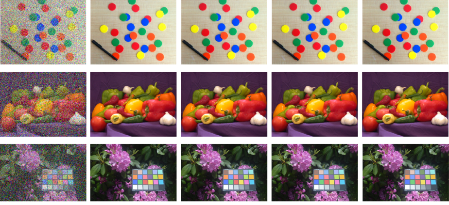
The restored images of ColoredChips, Peppers and ColorChecker with 20% salt-and-pepper noise by ITTPRP method, IRTTPRP method, TTPRP method and IDLA method are displayed respectively from left to right.
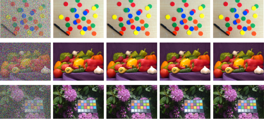
The restored images of ColoredChips, Peppers and ColorChecker with 40% salt-and-pepper noise by ITTPRP method, IRTTPRP method, TTPRP method and IDLA method are displayed respectively from left to right.
The restored images of ColoredChips, Peppers and ColorChecker with 60% salt-and-pepper noise by ITTPRP method, IRTTPRP method, TTPRP method and IDLA method are displayed respectively from left to right.
20% noise
Peppers
ColoredChips
ColarChecker
ITTPRP
39.25
39.60
40.71
IRTTPRP
39.36
39.52
40.62
TTPRP
39.18
39.40
40.60
IDLA
39.11
39.51
41.09
40% noise
Peppers
ColoredChips
ColarChecker
ITTPRP
34.72
34.79
36.27
IRTTPRP
34.60
34.80
36.29
TTPRP
34.52
34.56
36.22
IDLA
34.19
34.39
35.84
60% noise
Peppers
ColoredChips
ColarChecker
ITTPRP
31.24
31.13
32.81
IRTTPRP
31.22
31.12
32.75
TTPRP
30.87
30.35
32.72
IDLA
30.97
30.48
32.04
5 Conclusions
The primary contribution of this article is the proposal of an inertial three-term PRP CG projection method for large-scale nonlinear equations. This method achieves global convergence under appropriate assumptions. The experimental results demonstrate that the incorporation of the extrapolation strategy significantly accelerates the algorithm’s iteration. Furthermore, a comparison of various methods for image restoration problems clearly illustrates the superiority and effectiveness of the ITTPRP algorithm. This image restoration technique has the potential to enhance video surveillance, medical image processing, and various other practical applications, paving the way for further research and technological development.
CRediT authorship contribution statement
Gonglin Yuan: Writing – review & editing, Supervision, Funding acquisition. Chunzhao Liang: Writing – original draft, Visualization, Validation, Software, Resources, Methodology, Investigation, Formal analysis, Data curation, Conceptualization. Yong Li: Writing – review & editing, Supervision.
Acknowledgments
This work is supported by Guangxi Science and Technology base and Talent Project, PR China (Grant No. AD22080047), the major talent project of Guangxi (GXR-6BG242404), the special foundation for Guangxi Ba Gui Scholars, the Innovation Project of Guangxi Graduate Education, PR China (Grant No. YCBZ2024001), and the Guangxi Natural Science Foundation, PR China (Grant No. 2024GXNSFAA999149). Thanks to the editor and reviewers for their valuable comments, which greatly improved the quality of the paper.
Declaration of competing interest
The authors declare that they have no known competing financial interests or personal relationships that could have appeared to influence the work reported in this paper.
References
- Relaxed inertial Tseng’s type method for solving the inclusion problem with application to image restoration. Mathematics. 2020;8:818.
- [Google Scholar]
- Inertial iterative schemes with variable step sizes for variational inequality problem involving pseudomonotone operator. Mathematics. 2020;8:609.
- [Google Scholar]
- Solving nonlinear monotone operator equations via modified sr1 update. J. Appl. Math. Comput. 2021:1-31.
- [Google Scholar]
- An accelerated subgradient extragradient algorithm for strongly pseudomonotone variational inequality problems. Thai J. Math.. 2019;18:166-187.
- [Google Scholar]
- Weak convergence of a relaxed and inertial hybrid projection-proximal point algorithm for maximal monotone operators in Hilbert space. SIAM J. Optim.. 2004;14:773-782.
- [Google Scholar]
- An inertial proximal method for maximal monotone operators via discretization of a nonlinear oscillator with damping. Set-Valued Anal.. 2001;9:3-11.
- [Google Scholar]
- A logarithmic-quadratic proximal method for variational inequalities. In: Computational Optimization: A Tribute to Olvi Mangasarian. Vol vol. I. 1999. p. :31-40.
- [Google Scholar]
- Inertial proximal admm for linearly constrained separable convex optimization. SIAM J. Imaging Sci.. 2015;8:2239-2267.
- [Google Scholar]
- A global convergent quasi-Newton method for systems of monotone equations. J. Appl. Math. Comput.. 2014;44:455-465.
- [Google Scholar]
- A primal–dual fixed point algorithm for convex separable minimization with applications to image restoration. Inverse Problems. 2013;29:025011
- [Google Scholar]
- A finite element approximation for the initial-value problem for nonlinear second-order differential equations. J. Math. Anal. Appl.. 1985;111:90-104.
- [Google Scholar]
- A method with inertial extrapolation step for convex constrained monotone equations. J. Inequal. Appl.. 2021;2021:189.
- [Google Scholar]
- Iterative algorithm for triple-hierarchical constrained nonconvex optimization problem and its application to network bandwidth allocation. SIAM J. Optim.. 2012;22:862-878.
- [Google Scholar]
- A family of inertial derivative-free projection methods for constrained nonlinear pseudo-monotone equations with applications. Comput. Appl. Math.. 2022;41:309.
- [Google Scholar]
- Inertial extragradient method via viscosity approximation approach for solving equilibrium problem in Hilbert space. Optimization. 2021;70:387-412.
- [Google Scholar]
- A derivative-free rmil conjugate gradient projection method for convex constrained nonlinear monotone equations with applications in compressive sensing. Appl. Numer. Math.. 2021;165:431-441.
- [Google Scholar]
- A derivative-free iterative method for nonlinear monotone equations with convex constraints. Numer. Algorithms. 2019;82:245-262.
- [Google Scholar]
- A modified inertial three-term conjugate gradient projection method for constrained nonlinear equations with applications in compressed sensing. Numer. Algorithms. 2023;92:1621-1653.
- [Google Scholar]
- A methodology for solving chemical equilibrium systems. Appl. Math. Comput.. 1987;22:333-361.
- [Google Scholar]
- Inertial proximal alternating linearized minimization (ipalm) for nonconvex and nonsmooth problems. SIAM J. Imaging Sci.. 2016;9:1756-1787.
- [Google Scholar]
- Some methods of speeding up the convergence of iteration methods. USSR Comput. Math. Math. Phys.. 1964;4:1-17.
- [Google Scholar]
- Active-set projected trust-region algorithm for box-constrained nonsmooth equations. J. Optim. Theory Appl.. 2004;120:601-625.
- [Google Scholar]
- An efficient Dai-Yuan projection-based method with application in signal recovery. PLoS One. 2024;19:1-26.
- [Google Scholar]
- Two optimal Hager–Zhang conjugate gradient methods for solving monotone nonlinear equations. Appl. Numer. Math.. 2020;153:217-233.
- [Google Scholar]
- A new hybrid approach for solving large-scale monotone nonlinear equations. J. Math. Fundam. Sci.. 2020;52:17-26.
- [Google Scholar]
- An inertial Dai-Liao conjugate method for convex constrained monotone equations that avoids the direction of maximum magnification. J. Appl. Math. Comput.. 2024;70:4319-4351.
- [Google Scholar]
- A globally convergent inexact Newton method for systems of monotone equations. In: Reformulation: Nonsmooth, piecewise smooth, semismooth and smoothing methods. 1999. p. :355-369.
- [Google Scholar]
- Nonmonotone trust-region methods for bound-constrained semismooth equations with applications to nonlinear mixed complementarity problems. SIAM J. Optim.. 2001;11:889-917.
- [Google Scholar]
- A regularized semi-smooth newton method with projection steps for composite convex programs. J. Sci. Comput.. 2018;76:364-389.
- [Google Scholar]
- Non-smooth equations based method for 1-norm problems with applications to compressed sensing. Nonlinear Anal. TMA. 2011;74:3570-3577.
- [Google Scholar]
- A generalized hybrid cgpm-based algorithm for solving large-scale convex constrained equations with applications to image restoration. J. Comput. Appl. Math.. 2021;391:113423
- [Google Scholar]
- A hybrid three-term conjugate gradient projection method for constrained nonlinear monotone equations with applications. Numer. Algorithms. 2021;88:389-418.
- [Google Scholar]
- A family of inertial-relaxed dfpm-based algorithms for solving large-scale monotone nonlinear equations with application to sparse signal restoration. J. Comput. Appl. Math.. 2023;419:114674
- [Google Scholar]
- A three-terms Polak–Ribière–Polyak conjugate gradient algorithm for large-scale nonlinear equations. J. Comput. Appl. Math.. 2015;286:186-195.
- [Google Scholar]
- Limited memory bfgs method for nonlinear monotone equations. J. Comput. Math. 2007:89-96.
- [Google Scholar]
- A globally convergent bfgs method for nonlinear monotone equations without any merit functions. Math. Comp.. 2008;77:2231-2240.
- [Google Scholar]
- Superlinear convergence of a newton-type algorithm for monotone equations. J. Optim. Theory Appl.. 2005;125:205-221.
- [Google Scholar]


