A generalized model for quantitative analysis of sediments loss: A Caputo time fractional model

1 Introduction

Sediment loss and their transportation play a nominal role within the sedimentary basin because of natural hazards and climatic land erosions (Kaffas and Hrissanthou, 2019). To know the rate of sediment loss and it’s controlling and decaying factors, quantitative analysis based on the Caputo time the fractional model has significant importance in the mathematical studies (Caputo and Carcione, 2013). The mass of sediments can be discussed from different theories. Garrel and Mackenzie (Garrels and MacKenzie, 1972) present a theory called a constant mass model in which the total mass of sediments remains constant throughout the geological time. This theory postulates that there exists a balance between the metamorphism of sediments and erosion of igneous rocks, but the total mass of the sediments remains constant. Another theory is known as the linear accumulation model which stated that there is a higher rate of erosion of igneous rocks than the rate of formation of igneous mass. Furthermore, the sedimentary rocks could also be altered to igneous or metamorphic rocks.

The quantification of sediment loss by conventional methodologies are quite expensive and intensive labor activity is involved. Hence, the application of mathematical modeling is well supported to efficiently estimate the sediment loss in a sedimentary basin (Kaffas and Hrissanthou, 2019). Furthermore, the integration of the controlling factor (erosion rates) and time scale will highlight a variety of effects on the rate of sediment loss.

Sediment models can be classified into empirical, physical, or conceptual models. The classic empirical models are computationally swifter while conceptual models fit well for regional studies and longer temporal scale (DeMars et al., 2018). The loss of sediments is greatly dependent on its controlling factors, for instance, the rate of erosion, the mechanics of erosion, and the sediment transport processes (Foster and Meyer, 1975). The water in the form of rainfall not only acts as an agent of erosion but also contributes to the transport of sediments loss from the original rock mass (Williams, 1975). The controlling factor (erosion) is severely influenced by the rate of precipitation. Moreover, the erosion and sediment loss are differentially influenced by surface runoff, rainfall patterns, and the intensity of rainfall (Tao et al., 2017). Numerous sources in a sedimentary basin considerably influence the sediment loss. This process is better enlightened by the sediment delivery distributed (SEDD) model incorporates the factors of erosion and topography which are responsible for sediment loss mechanism in a given time frame (Ferro and Porto, 2000). Sarangi and Bhattacharya (2000, 2005) discussed the sediment loss with geomorphological constraints by a regression model that explains the loss of sediment concentration in runoff as a result of rainfall for the definite time interval. This model is quite useful in predicting the sediment loss per unit time which has quite precise data as compared to originally observed sediment yield. Yitian and Gu (2003) explained the sediment loss model with hydrological implications in rivers by using mass conservation transfer function. Boomer et al. (2008) found that the application of multiple regression models for estimating the sediment loss significantly deviates from the original observed data. They recommend the empirical and simulation models fit more precisely for controlling factors and sediment loss. Sediment delivery ratios based on the number of sediments concerning the area are estimated from the slope gradient, the roughness of the surface, moisture content, and the proximity of transporting pathways.

The prediction of sediment loss is modeled by regression models (Sarangi and Bhattacharya, 2000). However, the incorporation of geomorphological variables (including slope or relief and drainage pattern) significantly supports the prediction of sediment loss (Sarangi and Bhattacharya, 2005). The results from Boomer et al. (2008) suggested that to apply the multiple regression model for controlling factors of sediment yield, certain parameters of landscape-level should also be incorporated like the complexity of topographic surface, gradient or slope, and the rate of precipitation. Linear and polynomial regression analysis is a quite useful technique to calculate the sediment loss on a temporal scale and express a more realistic expression of sediment loss. The wide range of time from hourly to year, continuous assessment of controlling factor, and morphological profiling of a sedimentary basin are the key benefits of applying this mathematical model (Kaffas and Hrissanthou, 2019).

Fractional calculus has been growing nowadays vastly due to its versatile and unique properties. The non-integer order derivative is solved through fractional calculus tools. Fractional calculus is the extension of classical calculus and it has approximately three centuries-old histories. Fractional calculus is an important and fruitful tool for describing many systems including memory. In the last few years, fractional calculus is used for many purposes in various fields, such as electrochemistry, transportation of water in ground level, electromagnetism, elasticity, geology, diffusion, and in conduction of heat process. The most used fractional derivatives operator is the Caputo fractional derivative operator (Ali et al., 2017). A one-dimensional memory model for sediment diffusion in water reservoirs is studied by Caputo and Carcione (2013)They have used the Caputo fractional derivative operator for their analysis and concluded that fractional calculus is the best tool to describe the phenomenon. Chen et al. (2013) proposed a fractional model for sediment suspension in turbulence. They have described that the vertical distribution of sediments in the steady flow is well analyzed by the fractional model. In many complex real-world problems, fractional derivatives have been used, for instance, (Kumar et al., 2020a, 2020b, 2020c, 2020d, 2018; Sheikh et al., 2017; Sheikh, 2017; Yang, 2019; Singh, 2020a, 2020b; Singh et al., 2020, 2019).

Keeping in view the above literature survey and discussion, in this study the classical model of sediment loss is generalized using the concept of non-integer order derivatives namely, Caputo time-fractional derivatives. The generalized model is solved using the Laplace transformation technique and the solution is presented in terms of special function.

2 Mathematical modeling

Depending on the controlling factors the sediment loss occurs within the specified time interval. However, irrespective of the intensity of sediment loss, the total mass (initial sediments and newly formed sediments) will remain constant. It means that the rate of sediment loss is directly related to the deposition of new sediments. Harbaugh and Bonham-Carter (1970) suggested a model in which the quantity of material $M(t)$ loss by erosion (decaying parameter $\beta$ ) or (controlling factor $-\beta$ is rock competence or strength) per unit time $t$ is expressed by exponential decay equation (Ferguson, 1988)

To generate a generalized model for the sediment concentration, Fick’s first law (Caputo and Carcione, 2013) is used and we arrived at:

Applying the Laplace transformation to Eq. (3), using the initial condition from Eq. (2) we get

Inverting the Laplace transform of Eq. (5) the final solution is given by:

3 Special case

For $\alpha =1$ the corresponding solution (Ferguson, 1988) for the classical model is recovered as

4 Results and discussion

The study includes the parameters of sediment loss where the original mass of rock is represented by $M(t)$ while the controlling factor is mainly focused on rock strength or competence of rock. Only sedimentary rocks have been discussed in the work in which shales or mudstones are relatively incompetent lithology (less strength and lower value of controlling factor) whereas sandstone especially the thick to massive sandstones are considered as competent lithology (higher values of controlling parameter).

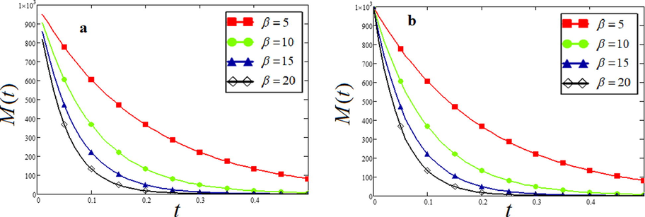
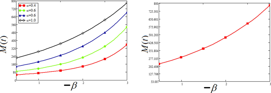
The relation between the reduction of mass (sediment loss) is a function of time where time is the independent variable and sediment loss is the dependent one. Mass reduction is directly related to time. However, the decaying parameter $\beta$ The decaying parameter is termed as weathering or erosion in this case. The extent of erosion adversely affects the mass reduction in unit time. Increasing the rate of erosion and weathering will significantly reduce the initial original mass in unit time. The values of erosion range from 5 to 20 in this study (Fig. 1) where 5 value of decay parameter (erosion) is least while 20 is the maximum limit of erosion. The rate of precipitation temperature changes will significantly increase the phenomenon of erosion. In Table 1 the comparison of exact solution and Zakian method is presented and a strong agreement between them is found for $\alpha =1$ , this agreement is also depicted from Fig. 1.

Close

Fig. 1

Plot of $M(t)$ against time for different values of the Decay parameter (weathering and erosion). The different rate of erosion determines the values of mass reduction in unit time. (a. Zakian method for Laplace inverse (Zakian, 1969), b. exact solution).

Export to PPT

The extent and variation of decaying parameter (weathering and erosion) vary from region to region. In this study, the decaying parameter os considered as an erosion factor. The agents of erosion (wind, water, and organisms) will determine the value of the decaying parameter $\beta$ Additionally, the climatic conditions and the intensity of erosion also influence the value of the decaying parameter. Generally, tropical climate conditions are more susceptible to weathering and erosion than semi-arid or arid regions (Jamil et al., 2020). It is therefore believed that the reduction of mass in unit time is primarily determined by decaying factor (weathering or erosion). From the figure, it is clear that $M(t)$ is decreasing with increasing time and decaying parameter.

Although it is challenging to apply the time parameter as a variable because the time in geological time usually ranges from thousand years to million years. Nevertheless, it is relatively convenient to see the changes in incompetent rocks (shales) as the weathering or erosion of shales happened more rapidly owing to low controlling factors. For this purpose, the geological fieldwork was planned in two phases to observe the reduction of mass of incompetent lithologies. With an increase in values of $\alpha$ , a rapid decaying behavior of $M(t)$ is noticed from Fig. 2From this figure, it is noticed that more than one plots can be drawn for the sediment loss even all the other physical parameters are kept constant, which is due to the memory effect of the fractional model. When we increase the values of $\beta$ at a fixed time $M(t)$ is showing a decreasing trend which means that $\beta$ is expediting the decaying process.

Close

Fig. 2

Plot of $M(t)$ against decay parameter for different values of the fractional parameter. (a. fractional solutions b. classical solution).

Export to PPT

The loss of sediments was noticed in geological fieldwork. The first phase of fieldwork was done during the fresh exposure of the outcrop section. This Kampung Kawang outcrop is selected for the study because it mainly comprised of shale (incompetent lithology) (Jamil et al., 2020) having a high value of sediment loss (decay parameter). The fresh exposure had a rare amount of mass reduction phenomenon (Fig. 3) as weathering and erosion has not influenced the outcrop section. However, in the second phase of geological fieldwork of the same outcrop reveal the sediment loss (weathered shale at the toe of outcrop). This weathered and eroded heap of shale or mud is an indication of rapid sediment loss from the original total mass. Large heaps of mud or shale are present at the base of the outcrop (Fig. 4). The comparative analysis of the Kawang section disclosed the higher fraction of sediment loss with an increase in the decay parameter.

Close

Fig. 3

The recent exposure of rocks due to infrastructure development of Pan Borneo highway. The time is considered near to zero. Even the rocks having lower values of controlling factor (shales) are intact and there is no clear evidence of sediment loss or sediment reduction. The field photograph was taken during the first phase of geological fieldwork in the Kawang road section, SW Sabah, Malaysia (Jamil et al., 2020, 2019).

Export to PPT

Close

Fig. 4

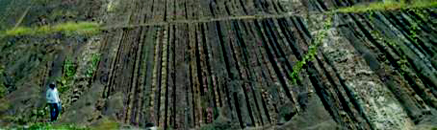
The time flies away, and we can see the loss of sediment. The second phase of the geological field in the same location outlines the effect of time in the real outcrop. The sediments having low controlling factors (incompetent shales) rapidly lose to decrease the initial value of mass. The reduction of mass with time is quite evident from this rock section. The field photograph was taken during the second field visit in the Kawang road section, SW Sabah, Malaysia.

Export to PPT

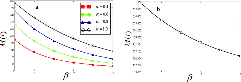
The relationship of time with sediment loss or decay parameter is extrapolated by using mathematical modeling. There exists a relation between the time and the decay parameter (sediment loss). Normally, the mass is gradually on the verge of reduction as the time increases. Geological processes eventually reduce the original mass that was deposited in a sedimentary basin. Nevertheless, it also depends on the rate of sediment loss (decay parameter) where higher sediment loss is attributed to the high reduction of the initial mass. The different values of rate of decay indicate the mass reduction concerning time values. There is a steep reduction of mass in case of high decay parameter (incompetent rocks) than the rocks having low values of decay parameter. The lower fraction of sediment loss is linked with the higher controlling factor (Fig. 5). The sandstone units having a high controlling factor remain intact with no sediment loss while the shale units (low controlling factor) eroded with the increase value of sediment loss. In this case, time is considered as constant both for shales and sandstone units.

Close

Fig. 5

The effect of controlling factor with sediment loss of initial mass. The empty of void spaces between the sandy intervals (visible as black lines) were previously sites of mudstones or shales units. These shales are readily lost in time due to low controlling factor while the sandstone units are intact, and no sediment loss occurs for the rocks having a high controlling factor. Keeping the time constant the effect of sediment loss is evident only on the mass having a low controlling factor. The field snap is taken from the University Prima Condo road section in Kota Kinabalu Sabah, Malaysia.

Export to PPT

Time plays a substantial role in sediment loss and resulted in the reduction of total original intact mass that was previously available in the form of outcrop or rock units. Although the mass with higher controlling factor offer resistant to decay or weather yet with an increase in the period, the sandstone having high controlling factor will start to disintegrate and contribute to the total sediment loss. Initially, the shale units (low controlling factor lithology) loss with the time but in a longer time interval, the resistant sandstone units start to weather and erode from the outcrop in form of blocks (Fig. 6). With the increase in time value, the sediment loss will definitely takes place even in rocks with high controlling factor.

Close

Fig. 6

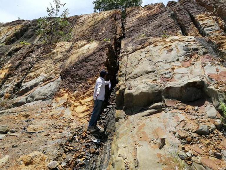
The increase in time values will not only decay the low controlling factor lithologies but also starts to erode the rocks having a high controlling factor. The author in the picture pointed out the space created due to decay (weathering and erosion) of shale (considered as an incompetent rock with low controlling parameter). Furthermore, the sand units overlying the eroded shale also weathered or decayed in the form of small blocks. This indicates that as we increase the time factor, both types of lithologies are differentially reduced in initial mass irrespective of their controlling factor. The field picture was taken from the outcrop section near University Utama outcrop near Telipok, NW Sabah, Malaysia.

Export to PPT

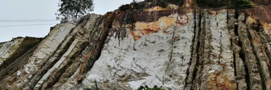
The increase in time values will not only result in complete loss of softer rocks (shale) but also influence the harder rocks (with high controlling factor). The sediment loss is quite visible in the sandstone outcrop in the form of a large number of blocks and a highly weathered sandstone section (Fig. 7). As the time values increase, it will contribute sufficiently to sediment loss both from shale and sandstone (irrespective of their controlling factor). Nevertheless, the rate of sediment is quite high in low controlling factor lithologies than the mass with a high controlling factor.

Close

Fig.7

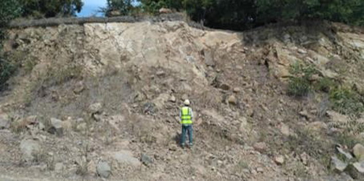
Represent the effect of time on high controlling parameter. The competent lithology (sandstone units) having high controlling factors are weathered or eroded with the increase in time values. In a longer time span, the reduction in sediments will significantly influence the rock with high controlling factors. The higher values of time are responsible for sediment loss even with high controlling factors. The field photograph was taken from Benoni Quarry in Sabah, Malaysia.

Export to PPT

There is a considerable loss of initial mass as the decay parameter come into the effect. The varying degree of decay parameter will determine the amount of sediments to be lost during the unit time. Higher decay parameter (weathering and erosion) will rapidly reduce the total mass while the low values of decay parameter ( $-\beta$ ) will gradual loss of sediments. Fig. 8 is drawn to show the effect of the controlling parameter on $M(t)$ It is clear from this figure that when we increase the magnitude of $-\beta$ , a greater value of $M(t)$ will remain at the fixed time.

Close

Fig. 8

Plot of $M(t)$ against controlling parameter for different values of the fractional parameter. (a. fractional solutions b. classical solution).

Export to PPT

5 Conclusion

In the present analysis, a mathematical model for sediment loss is proposed. A Caputo time-fractional derivative approach is used to generalize the model with the help of Fick’s first law. The exact solutions are obtained using the Laplace transform technique. The results are plotted in graphs and discussed in detail with the geological field images. The key points are as follow:

1. With varying time, the incompetent rocks (shales) readily decay within a brief span of time.

2. Keeping the time value constant, only incompetent rocks having a high decaying parameter will erode while competent rocks have less effect of the decaying parameter.

3. The significant time values, both the competent and incompetent lithologies tend to decay. However, the decay process is considerably more effective in the case of incompetent rocks.

4. For a single parameter, different plots can be drawn with several values of $\alpha$ , showing the memory effects which helps to inline the mathematical model with the geological processes.

The application of fractional calculus on a geoscientific phenomenon is discussed in this study in detail, which may provide a base for future studies. The model can be more generalized using the other definitions of fractional derivatives, like Caputo Fabrizio fractional derivatives and Atangana-Baleanu fractional derivatives. The idea of fractal-fractional calculus may also be considered in the future to predict the sedimentary processes more efficiently.

References

- Computation of hourly sediment discharges and annual sediment yields by means of two soil erosion models in a mountainous basin. Int. J. River Basin Manage.. 2019;17(1):63-77.
- [Google Scholar]
- Integrating GLEAMS sedimentation into RZWQM for pesticide sorbed sediment runoff modeling. Environ. Modell. Software. 2018;109:390-401.
- Mathematical simulation of upland erosion by fundamental erosion mechanics. In: Present and Prospective Technology for Predicting Sediment Yields and Sources. Vol vol. 40. New Orleans, LA: USDA_ARS Southern Region; 1975. p. :190-207.
- Sediment routing for agricultural watersheds 1. JAWRA J. Am. Water Resour. Assoc.. 1975;11(5):965-974.
- Mathematical model of sediment and solute transport along slope land in different rainfall pattern conditions. Sci. Rep.. 2017;7:44082.
- Use of geomorphological parameters for sediment yield prediction from watersheds. J. Soil Water Conserv.. 2000;44:99-106.
- Comparison of artificial neural network and regression models for sediment loss prediction from Banha watershed in India. Agric. Water Manage.. 2005;78(3):195-208.
- Modeling flow and sediment transport in a river system using an artificial neural network. Environ. Manage.. 2003;31(1):0122-0134.
- Empirical models based on the universal soil loss equation fail to predict sediment discharges from Chesapeake Bay catchments. J. Environ. Qual.. 2008;37(1):79-89.
- Magnetic field effect on blood flow of Casson fluid in axisymmetric cylindrical tube: a fractional model. J. Magn. Magn. Mater.. 2017;423:327-336.
- Fractional dispersion equation for sediment suspension. J. Hydrol.. 2013;491:13-22.
- An efficient numerical scheme for fractional model of HIV-1 infection of CD4+ T-cells with the effect of antiviral drug therapy. Alexandria Eng. J. 2020
- A modified analytical approach with existence and uniqueness for fractional Cauchy reaction–diffusion equations. Adv. Diff. Eqn.. 2020;2020(1):1-18.
- A new Rabotnov fractional-exponential function-based fractional derivative for diffusion equation under external force. Math. Methods Appl. Sci.. 2020;43(7):4460-4471.
- A study of fractional Lotka-Volterra population model using Haar wavelet and Adams-Bashforth-Moulton methods. Math. Methods Appl. Sci.. 2020;43(8):5564-5578.
- A comparative study of Atangana-Baleanu and Caputo-Fabrizio fractional derivatives to the convective flow of a generalized Casson fluid. Eur. Phys. J. Plus. 2017;132(1):54.
- Comparison and analysis of the Atangana-Baleanu and Caputo-Fabrizio fractional derivatives for generalized Casson fluid model with heat generation and chemical reaction. Results Phys.. 2017;7:789-800.
- General fractional derivatives: theory, methods and applications. CRC Press; 2019.
- Numerical simulation for fractional delay differential equations. Int. J.Dyn. Control 2020:1-12.
- Analysis for fractional dynamics of Ebola virus model. Chaos, Solitons Fractals. 2020;138:109992
- Effect of Hall current on the magnetohydrodynamic free convective flow between vertical walls with induced magnetic field. Eur. Phys. J. Plus. 2018;133(5):207.
- Legendre spectral method for the fractional Bratu problem. Math Methods Appl. Sci.. 2020;43(9):5941-5952.
- Solving non-linear fractional variational problems using Jacobi polynomials. Mathematics. 2019;7(3):224.
- Harbaugh, J.W., Bonham-Carter, G., 1970. Computer Simulation in Geology. Stanford Univ Calif.
- Geological applications of differential equations. In: Mathematics in Geology. Springer; 1988. p. :216-237.
- A new model of fractional Casson fluid based on generalized Fick’s and Fourier’s laws together with heat and mass transfer. Alexandria Eng. J. 2019
- Fractional relaxation-oscillation and fractional diffusion-wave phenomena. Chaos, Solitons Fractals. 1996;7(9):1461-1477.
- “A contemporary review of sedimentological and stratigraphic framework of the Late Paleogene deep marine sedimentary successions of West Sabah, North-West Borneo. Bull. Geol. Soc. Malaysia. 2020;69(1):53-65.
- Deep marine Paleogene sedimentary sequences of West Sabah: contemporary opinions and imbiquities. Warta Geol.. 2019;45(3):198-200.