

Translate this page into:
A parametrized approach to generalized fractional integral inequalities: Hermite–Hadamard and Maclaurin variants
⁎Corresponding author at: Department of Mathematics, Faculty of Arts and Sciences, Çankaya University, Ankara 06790, Turkey. fahd@cankaya.edu.tr (Fahd Jarad)
-
Received: ,
Accepted: ,
This article was originally published by Elsevier and was migrated to Scientific Scholar after the change of Publisher.
Abstract
This paper introduces a novel parametrized integral identity that forms the basis for deriving a comprehensive class of generalized fractional integral inequalities. Building on recent advancements in fractional calculus, particularly in conformable fractional integrals, our approach offers a unified framework for various known inequalities. The novelty of this work lies in its ability to generate new and more general inequalities, including Hermite–Hadamard-, Maclaurin-, and corrected Maclaurin-type inequalities, by selecting specific parameter values. These results extend the scope of fractional integral inequalities and provide new insights into their structure. To demonstrate the practical applicability and accuracy of the theoretical findings, we present a detailed numerical example along with graphical representations.
Keywords
65D32
26A45
26D10
26D15
Conformable fractional integral operators
Maclaurin-type inequalities
Corrected Maclaurin-type inequalities
Hermite–Hadamard-type inequalities
Convex functions

Data availability
Data sharing is not relevant to this article, as there was no generation or analysis of new data during the course of this study.
1 Introduction
In classical error estimations for quadrature formulas, the accuracy of the approximation improves as more points are included, often involving higher-order derivatives of the function. However, this approach faces challenges when the function is not sufficiently smooth or differentiable to the required order. The concept of convexity is of utmost importance in this context because it enables the formulation of integral inequalities that depend solely on the first- or second-order derivative, eliminating the requirement for higher-order differentiability. Using the characteristics of convex functions, it becomes feasible to calculate precise error estimations involving lower-order derivative terms; see Liu et al. (2023), Meftah et al. (2022), Meftah and Lakhdari (2023), Saleh et al. (2023b, c).
Let us recall that a function is considered convex on an interval if, for all , and , the following inequality holds:
Among the three-point quadrature formulas, Simpson’s rule is the most well known. However, Simpson’s rule, like many other closed quadrature formulas, is not effective for integrals where the function values at the endpoints are not well defined or when the endpoints contain singularities. In such situations, open-quadrature formulas are typically employed. One notable example of an open quadrature formula is the Maclaurin formula, which is given by
The Maclaurin formula approximates the integral by evaluating the function at three points within the interval , thus avoiding potential issues at the boundaries. This makes it particularly useful for integrals with undefined or problematic values at the endpoints, providing a reliable approximation method in such cases.
In Meftah and Allel (2022), the authors established the following Maclaurin inequality: where is convex on .
By extending the concept of integrals and derivatives to non-integer orders, fractional calculus provides a comprehensive framework for the analysis of functions with intricate, memory-dependent behavior. The Riemann–Liouville fractional integral is one of the most prominent definitions of fractional integrals. It extends the standard integral to fractional orders, thereby offering a potent instrument for the examination of functions that exhibit fractional-order dynamics.
Definition 1.1 Samko et al., 1993
The left- and right-sided Riemann–Liouville fractional integrals and of order are defined by respectively, where is the gamma function.
The above defined integrals have been crucial in the development of a variety of integral inequalities that generalize classical results to the fractional setting. These inequalities are essential for the development of numerical methods for fractional-order systems and the comprehension of the behavior of solutions to fractional differential equations. Researchers have developed new error estimates and bounds that expand on conventional findings, thereby offering a more comprehensive understanding of the fractional calculus framework; see Lakhdari and Meftah (2022), Saleh et al. (2023a), Xu et al. (2022) and the references cited therein.
The authors in Djenaoui and Meftah (2023) provided the fractional analogue of Maclaurin’s inequality via Riemann–Liouville integrals as follows:
where
The Riemann–Liouville operators have indeed been instrumental in uncovering hidden dynamics within complex systems. However, the unique characteristics exhibited by some nonlocal systems often escape the descriptive power of existing fractional integrals and derivatives. To better describe specific physical phenomena, many researchers have focused on developing alternative types of fractional operators, opening new avenues of research. This has led to numerous advancements in the field of integral inequalities, particularly through the use of Katugampola integrals (Lakhdari et al., 2024), fractional integrals with exponential kernels (Li et al., 2024), Caputo–Fabrizio integrals (Yasin et al., 2024), AB-fractional integrals (Yuan et al., 2023), -fractional Hilfer–Katugampola integrals (Naz et al., 2021b,a; Naz and Naeem, 2021), and discrete fractional sum (Naz and Chu, 2022), among others.
In Jarad et al. (2017), Jarad et al. proposed generalized fractional integral operators, achieved through the successive application of conformable integrals. These operators share several attributes with traditional fractional integrals and can be reduced to familiar forms such as the Riemann–Liouville and Hadamard integrals. The introduction of these operators offers new insight into fractional variational problems, optimal control issues, and the modeling of complex systems. Notably, these operators feature a dependence on two parameters, which enhances their ability to detect memory effects within the system. The conformable fractional integral operators are defined as follows:
Definition 1.2 Jarad et al., 2017
The left- and right-sided conformable fractional integrals of order with and are defined respectively by
Note that for , the generalized conformable integrals given in Definition 1.2 reduce to the Riemann–Liouville fractional integrals presented in Definition 1.1.
Recent advancements in conformable fractional calculus have led to significant contributions in the field of integral inequalities. In Hezenci and Budak (2023a), Hezenci and Budak explored trapezoid-type inequalities, while Kara et al. investigated midpoint-type and trapezoidal-type inequalities for twice-differentiable functions in Kara et al. (2023). Furthermore, Hezenci and Budak presented Simpson-type inequalities in Hezenci and Budak (2023b), and Unal et al. examined Newton-type inequalities for differentiable convex functions in Ünal et al. (2023). Set et al. introduced Ostrowski-type inequalities in Set et al. (2019), and studied Hermite–Hadamard-type inequalities in Set et al. (2021). Further contributions include Rashid et al. on Minkowski inequalities (Rashid et al., 2020), and Hyder et al. on midpoint inequalities (Hyder et al., 2021). Rahman et al. also made significant contributions with studies on Grüss-type and Chebyshev-type inequalities in Rahman et al. (2018) and Rahman et al. (2019), respectively. These works collectively advance the understanding and application of conformable fractional integrals in mathematical analysis. For more works, we refer the readers to Nisar et al. (2019), Ying et al. (2024), Zhou and Du (2023).
Motivated by the importance and utility of the generalized fractional integrals introduced in Jarad et al. (2017), and inspired by the aforementioned works, in this paper, we introduce a new parametrized integral identity that will serve as the foundation for establishing some new conformable fractional Maclaurin-like inequalities for differentiable convex functions. Our findings provide a unifying framework, as for constant values of the identity’s parameter, we derive novel Maclaurin-, corrected Maclaurin-, as well as Hermite–Hadamard-type inequalities. The research concludes with an illustrative example confirming the correctness of the obtained results.
2 Auxiliary result
This section introduces a new integral identity related to conformable fractional integrals, which will serve as the main tool for establishing our results.
Let
be a differentiable function on
,
with
. If
, then for
,
, and
, the following equality holds
where
3 Primary results
This section presents the main results of our study.
Let be as in Lemma 2.1. If is convex on , then we have where , and are defined as in (2.1), (3.3) and (3.4) respectively, and and are the beta and the incomplete beta function, respectively.
Taking the absolute value in both sides of the equality given in Lemma 2.1, then using the convexity of , we get
where we have used the facts that
By setting , Theorem 3.1 gives where is defined as in (1.1).
In Corollary 3.2, if we take , we get
Let be as in Lemma 2.1. If is convex on where with , then we have where and are defined as in (2.1) and (3.5), respectively, and is the beta function.
From Lemma 2.1, Hölder’s inequality and convexity of
, we deduce
where we have used
By setting , Theorem 3.4 gives where is defined as in (1.1).
In Corollary 3.5, if we take , we get
Let be as in Lemma 2.1. If is convex on where , then we have where , and are defined as in (2.1), (3.3) and (3.4) respectively.
From Lemma 2.1, power mean inequality and the convexity of , we get where we have used (3.1)–(3.4) and (3.6) and Theorem 3.7. The proof is finished. □
By setting , Theorem 3.4 gives where is defined as in (1.1).
In Corollary 3.8, if we take , we get
4 Special cases
In this section, we derive several results related to some well-known quadrature rules.
In Theorem 3.1, if we take , we get the following Hermite–Hadamard-type inequality for conformable fractional integrals Moreover, if we set , we get Furthermore, if we take , we get
In Theorem 3.1, if we take , we obtained the following conformable fractional Maclaurin inequality
Here are some observations from Corollary 4.2:
-
By setting , Corollary 4.2 becomes equivalent to Corollary 2.1 in Djenaoui and Meftah (2023).
-
When and are both set to 1, Corollary 4.2 enhances the result presented by Meftah and Allel in Corollary 3.3 from Meftah and Allel (2022), as their result can be deduced by leveraging the convexity of .
In Theorem 3.1, if we take , we obtained the following conformable fractional Corrected Maclaurin inequality Moreover, if we choose , we get Furthermore, if we take , we obtain
As with Theorem 3.1, numerous special cases can be derived from Theorems 3.4 and 3.7 by setting specific values of .
5 Illustrative example
In this section, we present a numerical example with graphical representations to confirm the accuracy of our results.
Consider the function , defined by . The derivative of this function satisfies the basic condition of our results. Indeed, we have , which is convex on the interval .
The considered function yields:
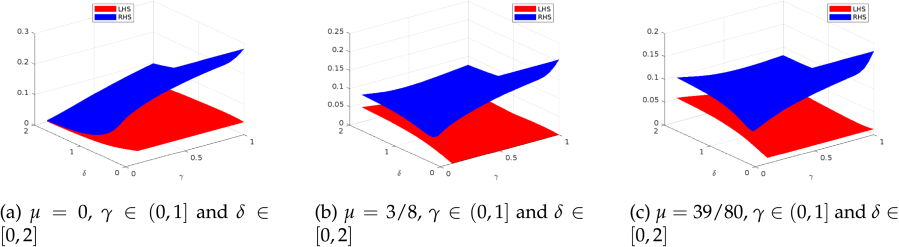
Now, in order to graphically represent the LHS and RHS, which depend on three parameters, we need to fix one of these parameters and plot the two quantities as functions of the remaining two parameters in turn.
Case.1 Let us begin by fixing the parameter . Some examples for , , and are depicted by Figs. 1(a), 1(b), and 1(c).
Case.2 Now, let us fix the parameter . The result related to the parametrized Riemann–Liouville fractional integrals is depicted in Fig. 2.
- Case.1.
Based on the different representations provided in Figs. 1 and 2, we observe that the left-hand side consistently lies below the right-hand side, which validates the accuracy of our results.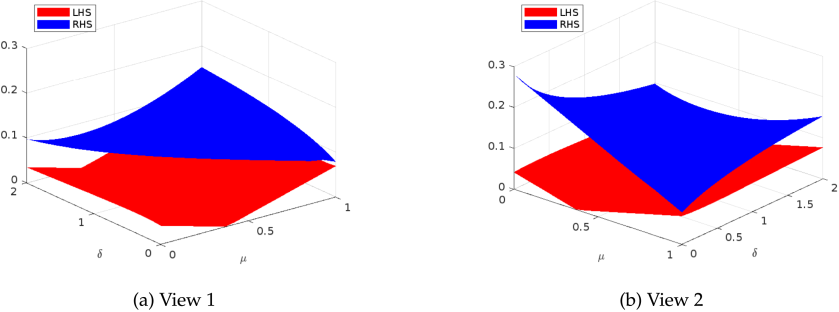
Case.2.
6 Conclusion
In this paper, we have developed a novel parametrized identity that significantly broadens the scope of fractional integral inequalities. The key contribution of this work is the unification of several well-known inequalities through a single framework, which not only encompasses classical results such as Hermite–Hadamard and Maclaurin-type inequalities but also yields new, more generalized versions. By introducing new parameters, our results offer greater flexibility and wider applicability in both pure and applied mathematics. The numerical examples and graphical representations provided serve to validate the correctness and effectiveness of our theoretical results. Future research may explore additional applications of these generalized inequalities across various fields, further enhancing their utility in solving complex mathematical problems.
CRediT authorship contribution statement
Abdelghani Lakhdari: Writing – review & editing, Writing – original draft, Software, Project administration, Investigation, Formal analysis, Conceptualization. Bandar Bin-Mohsin: Writing – review & editing, Writing – original draft, Project administration, Methodology, Investigation, Formal analysis, Conceptualization. Fahd Jarad: Writing – review & editing, Visualization, Supervision, Methodology, Conceptualization. Hongyan Xu: Writing – review & editing, Visualization, Validation, Methodology, Formal analysis. Badreddine Meftah: Writing – review & editing, Visualization, Validation, Supervision, Methodology.
Declaration of Generative AI and AI-assisted technologies in the writing process
During the preparation of this work, the authors used artificial intelligence tools to enhance language and readability. After generating the initial content with this AI, the authors carefully reviewed, edited, and refined the text to ensure accuracy and appropriateness for publication. The authors assume full responsibility for the final version of the manuscript.
Funding
No funding was received for this work.
Acknowledgment
This research is supported by Researchers Supporting Project Number (RSP2024R158), King Saud University, Riyadh, Saudi Arabia .
Declaration of competing interest
The authors declare that they have no known competing financial interests or personal relationships that could have appeared to influence the work reported in this paper.
References
- Fractional Maclaurin type inequalities for functions whose first derivatives are -convex functions. Jordan J. Math. Stat.. 2023;16(3):483-506.
- [Google Scholar]
- Novel results on trapezoid-type inequalities for conformable fractional integrals. Turkish J. Math.. 2023;47(2):425-438.
- [Google Scholar]
- Simpson-type inequalities for conformable fractional operators with respect to twice-differentiable functions. J. Math. Ext.. 2023;17
- [Google Scholar]
- Further integral inequalities through some generalized fractional integral operators. Fractal fract.. 2021;5(4):282.
- [Google Scholar]
- On a new class of fractional operators. Adv. Difference Equ. 2017:16. Paper No. 247
- [Google Scholar]
- A study on the new class of inequalities of midpoint-type and trapezoidal-type based on twice differentiable functions with conformable operators. J. Funct. Spaces 20234624604 11pp
- [Google Scholar]
- Extension of Milne-type inequalities to katugampola fractional integrals. Bound. Value Probl. 2024:16. Paper No. 100
- [Google Scholar]
- Some fractional weighted trapezoid type inequalities for preinvex functions. Int. J. Nonlinear Anal. Appl.. 2022;13(1):3567-3587.
- [Google Scholar]
- Further Hermite–Hadamard-type inequalities for fractional integrals with exponential kernels. Fractal Fract.. 2024;8(6):345.
- [Google Scholar]
- Some interesting inequalities for the class of generalized convex functions of higher order. J. Funct. Spaces 20234759187 10pp
- [Google Scholar]
- Maclaurin’s inequalities for functions whose first derivatives are preinvex. J. Math. Anal. Model.. 2022;3(2):52-64.
- [Google Scholar]
- Dual simpson type inequalities for multiplicatively convex functions. Filomat. 2023;37(22):7673-7683.
- [Google Scholar]
- Some new Hermite–Hadamard type integral inequalities for twice differentiable s-convex functions. Comput. Math. Model.. 2022;33(3):330-353.
- [Google Scholar]
- A unified approach for novel estimates of inequalities via discrete fractional calculus techniques. Alex. Eng. J.. 2022;61(1):847-854.
- [Google Scholar]
- New generalized reverse Minkowski inequality and related integral inequalities via generalized -fractional Hilfer-Katugampola derivative. Punjab Univ. J. Math. (Lahore). 2021;53(4):247-260.
- [Google Scholar]
- Ostrowski-type inequalities for -polynomial -convex function for -fractional Hilfer-Katugampola derivative. J. Inequal. Appl. 2021:23. Paper No. 117
- [Google Scholar]
- Some -fractional extension of Grüss-type inequalities via generalized Hilfer-Katugampola derivative. Adv. Difference Equ. 2021:16. Paper No. 29
- [Google Scholar]
- Some inequalities via fractional conformable integral operators. J. Inequal. Appl. 2019:8. Paper No. 217
- [Google Scholar]
- Some new inequalities of the Grüss type for conformable fractional integrals. AIMS Math.. 2018;3(4):575-583.
- [Google Scholar]
- Certain Chebyshev-type inequalities involving fractional conformable integral operators. Mathematics. 2019;7(4):364.
- [Google Scholar]
- New generalized reverse Minkowski and related integral inequalities involving generalized fractional conformable integrals. J. Inequal. Appl. 2020:15. Paper No. 177
- [Google Scholar]
- On fractional biparameterized Newton-type inequalities. J. Inequal. Appl. 2023:18. Paper No. 122
- [Google Scholar]
- Some remarks on local fractional integral inequalities involving Mittag–Leffler kernel using generalized -convexity. Mathematics. 2023;11(6):1373.
- [Google Scholar]
- Quantum dual Simpson type inequalities for q-differentiable convex functions. Int. J. Nonlinear Anal. Appl.. 2023;14(4):63-76.
- [Google Scholar]
- Fractional integrals and derivatives. In: Theory and Applications. Yverdon: Gordon and Breach Science Publishers; 1993. Edited and with a foreword by S. M. Nikol’skiĭ. Translated from the 1987 Russian original. Revised by the authors
- [Google Scholar]
- Ostrowski type inequalities via new fractional conformable integrals. AIMS Math.. 2019;4(6):1684-1697.
- [Google Scholar]
- Hermite–Hadamard type inequalities involving nonlocal conformable fractional integrals. Malays. J. Math. Sci.. 2021;15(1):33-43.
- [Google Scholar]
- Conformable fractional Newton-type inequalities with respect to differentiable convex functions. J. Inequal. Appl. 2023:19. Paper No. 85
- [Google Scholar]
- Fractional versions of Hermite–Hadamard, Fejér, and Schur type inequalities for strongly nonconvex functions. J. Funct. Spaces 20227361558 8pp
- [Google Scholar]
- Hermite–Hadamard type inequality for non-convex functions employing the Caputo–Fabrizio fractional integral. Res. Math.. 2024;11(1):10. Paper No. 2366164
- [Google Scholar]
- Simpson-like inequalities for twice differentiable (s, p)-convex mappings involving with AB-fractional integrals and their applications. Fractals. 2023;31(03):2350024
- [Google Scholar]
- On the reverse Minkowski’s, reverse Hölder’s and other fractional integral inclusions arising from interval-valued mappings. IAENG Int. J. Appl. Math.. 2023;53(4):1-14.
- [Google Scholar]


