Global stability and modeling with a non-singular kernel for fractional order heroin epidemic model: Insights from different population studies

Miguel Vivas-Cortez; Abu Bakar; M.S. Alqarni; Nauman Raza; Talat Nazir; Muhammad Farman

doi:10.1016/j.jksus.2024.103329

View/Download PDF

Buy Reprints

PDF

Translate this page into:

Full Length Article

10 2024

:36;

103329

doi:

10.1016/j.jksus.2024.103329

Global stability and modeling with a non-singular kernel for fractional order heroin epidemic model: Insights from different population studies

Miguel Vivas-Cortez^a, Abu Bakar^b, M.S. Alqarni^c, Nauman Raza^d,e, Talat Nazir^f,⁎, Muhammad Farman^e,g

a School of Physical and Mathematical Sciences, Faculty of Exact and Natural Sciences, Pontificia Universidad Católica del Ecuador, Av. 12 de Octubre 1076, Apartado, Quito 17-01-2184, Ecuador

b Research Centre on Public Health (CESP), Department of Medicine and Surgery, University of Milan-Bicocca, Monza, Italy

c Department of Mathematics, College of Science, King Khalid University, P.O. Box 9004, Abha 61413, Saudi Arabia

d Department of Mathematics, University of the Punjab, Quaid-e-Azam Campus, Lahore, Pakistan

e Department of Mathematics, Near East University, TRNC, Mersin 10, Nicosia 99138, Turkey

f Department of Mathematical Sciences, University of South Africa, Florida 0003, South Africa

g Department of Computer Science and Mathematics, Lebanese American University, 1107-2020, Beirut, Lebanon

⁎Corresponding author. talatn@unisa.ac.za (Talat Nazir)

Received: 2024-2-16, Accepted: 2024-6-26,

Disclaimer:
This article was originally published by Elsevier and was migrated to Scientific Scholar after the change of Publisher.

Abstract

There has been a worldwide epidemic of heroin that has affected people, families, societies, and cultures across the world. Now, the heroin epidemic has transitioned from heroin abuse to the overuse of synthetic narcotics, which are widely accessible and inexpensively produced. In this work, a novel mathematical approach is applied to investigate the dynamics of the heroin epidemic model and its harmful effect on society with different population data. A heroin model has been constructed with the importance of a non-singular kernel in the sense of a generalized Mittag-Leffler kernel. The well-posedness of the proposed model is proven via fixed-point theory. To examine the heroin model, two equilibrium states have been determined. These equilibrium states are proven to be locally and globally asymptotically stable. To analyze the behavior of heroin, a basic reproduction number and sensitivity analysis are used to determine the impact of different parameters mathematically as well as through simulations. To find the approximate solution, we implement the Toufik–Atangana numerical method at different fractional order values. The sensitivity of the heroin model is carried out, and 3-D graphs show the significance of the parameter involved in the model. Finally, the numerical outcomes are presented with different values of fractional parameters.

Keywords

Heroin epidemic model

Atangana–Baleanu fractional derivative

Sensitivity analysis

Stability

Numerical solution

Show Related Articles from PubMed

Data availability

Our manuscript has no associated data.

1 Introduction

The escalating intake of drugs and other dangerous substances is a severe concern. Heroin addiction affects not just the level of life for the vast majority of people but also, to a greater extent, the overall picture of world peace and economic prosperity (Xu, 2023; Glicksberg et al., 2023). Based on data from the United Nations (U.N.) World Drug Report, 35 million people have severe problems related to drug misuse, and only around a seventh are receiving a cure (Fabien, 2018). In addition, it was disclosed that drug addiction occurred globally in 2017, with 3 million cases of HIV and 6.2 million cases of severe hepatitis B viral infections. Metric records indicate that the detrimental physiological effects of drug use are more widespread and substantial than previously thought and that controlling the prevalence of harmful drugs is essential (Saha and Samanta, 2019; Tolomeo et al., 2021).

An indispensable mechanism for comprehending and treating drug addiction challenges is mathematically modeled (Raza et al., 2023). It has come to light that models are beneficial tools for forecasting drug users’ behavior patterns and offering practical recommendations for therapeutic approaches (Chou and D’Orsogna, 2022; Raza et al., 2022b). Narcotic drug misuse, including heroin consumption, is already a major societal issue. Wangari and Stone (2017) have investigated the spread of heroin addiction in society with the saturated treatment function. Zhang and Xing (2020) have formulated a reaction–diffusion heroin disease model with stability analysis. The authors in Huang and Liu (2013) proposed a distributed delay model of heroin and examined the dynamics in the population. In Liu and Wang (2016), the authors have modeled the heroin model with the saturating rate of non-linear occurrence and provided conditions for the global disease dynamics. Khan et al. (2021) have discussed preferable control factors for heroin spread with sensitivity.

A noteworthy advancement has recently been made in fractional calculus, using new derivative and integral operators with kernels (Butt et al., 2023a,c; Zafar et al., 2021 ). The creatively suggested element takes advantage of a modified version of the Mittag-Leffler function (MLF), this structure encompasses the keystone and its properties, which play a vital role in developing innovative methods to attain various fascinating characteristics, like the expanding variations and mean square deformation interphase that are found in significant scenarios. The authors in Zafar et al. (2021) developed a heroin model using a fractional operator. Weera et al. (2023) have considered a fractional heroin model for the numerical solutions. The groundbreaking fractional derivative operator, developed by Atangana and Baleanu in 2016, has widespread use in several scientific and technological fields. It has been demonstrated that utilizing the AB-fractional operator in simulation produces a disordered framework. for a brief time (Syam and Al-Refai, 2019; Bas and Ozarslan, 2018; Gomez-Aguilar et al., 2016; Owolabi and Atangana, 2019 ). The AB-fractional derivative is an excellent mathematical method for modeling progressively complex critical difficulties in the setting of Caputo since it has now been found that the MLF is a more significant and effective filtering procedure than the exponential and power laws.

In this work, we develop an epidemic model of heroin comprising addiction and enduring immunity, then explore the worldwide patterns triggered by the previous arguments. We used the new ABC-fractional method and Toufik–Atangana’s approach (Mekkaoui and Atangana, 2017) to create a fractional representation and evaluate numerical results. To the researchers knowledge, a few studies have used the ABC-fractional operator to analyze the heroin epidemic scenario. Additionally, the researchers claim that there is an absence of appropriate research that examines robust management of computational structures from the standpoint of ABC-fractional forms.

The paper’s structure is as follows: In Section 2, we delve into the dynamics of heroin, providing detailed explanations and introducing fundamental concepts in fractional calculus. Moving on to Section 3, we demonstrate the model’s existence and uniqueness using mathematical approaches. Section 4 is dedicated to analyzing the model’s stability analytically. Section 5 covers the numerical method and its corresponding results. Finally, Section 6 offers insights into the research’s overall conclusions.

2 Formulation and configuration of heroin model

This section outlines the creation of the heroin disease epidemic model (Raza et al., 2022a), and three subgroups comprise the whole population. $U (t)$ represents susceptible persons, $V (t)$ shows drug users, and $W (t)$ displays non-drug users, which are the state variables in the model, respectively. This model considers the following assumptions:

The total population $N$ is the sum of all the subclasses and its size is assumed to be fixed in the whole period.
All the biological parameters must be nonnegative or positive.
Homogeneous mixing is considered.
All of the individuals are supposed to be identically susceptible to drug habit.

Therefore, the heroin epidemic’s expansion is visualized in Fig. 1, and it is elucidated through the accompanying set of ODEs:

(1)

\{\begin{matrix} \frac{d U}{d t} & = & η - \frac{σ_{1} U V}{N} - δ_{1} U, \\ \frac{d V}{d t} & = & \frac{σ_{1} U V}{N} - ρ V + \frac{σ_{2} V W}{N} - δ_{1} V, \\ \frac{d W}{d t} & = & ρ V - \frac{σ_{2} V W}{N} - δ_{1} W, \end{matrix}

subject to initial conditions

U_{0} \geq 0, V_{0} \geq 0, W_{0} \geq 0

and

N = U + V + W

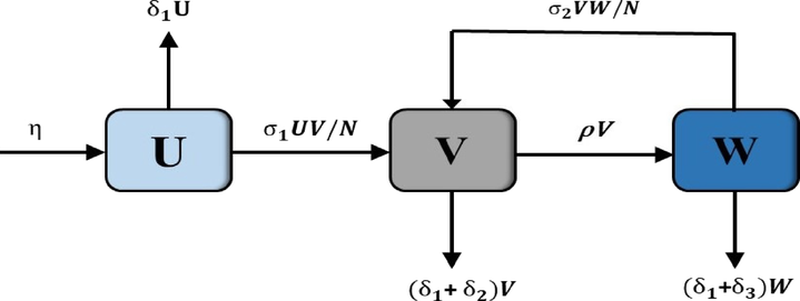
The heroin epidemic’s expansion within sub populations.

Due to the complex structure of the population, we equalize the system (1) by subsidizing the state variables: $S = \frac{U}{N}, X = \frac{V}{N}, Y = \frac{W}{N}$ as follows

(2)

\{\begin{matrix} \frac{d S (t)}{d t} & = & η - σ_{1} S X - δ_{1} S, t \geq 0, \\ \frac{d X (t)}{d t} & = & σ_{1} S X - ρ X + σ_{2} X Y - δ_{1} X, t \geq 0, \\ \frac{d Y (t)}{d t} & = & ρ X - σ_{2} X Y - δ_{1} Y, t \geq 0, \end{matrix}

with initial conditions

S_{0} \geq 0, X_{0} \geq 0, Y_{0} \geq 0

and

S (t) + X (t) + Y (t) = 1

. An elaborate explanation of the parameters employed in the study, along with a description of their scientific significance and relationship to certain physical occurrences to be provided in Table 1.

The traditional derivative neglects memory effects that exist in numerous biological structures. Therefore, We employ the Atangana–Baleanu fractional derivative in place of the conventional integer-order derivative in order to enlarge framework (2) for the present study. This transformation will enable us to track memory effects and get further insights into the dynamics of the heroin epidemic. Before continuing, we revisit key aspects of Atangana–Baleanu and Caputo derivatives (Butt et al., 2023b; Abdeljawad and Baleanu, 2017; Rashid et al., 2022; Butt et al., 2022 ).

Table 1 Interpretation of parameters of the heroin model.

Parameter	Interpretation
$η$	New drug users
$σ_{1}$	Probability rate of infection
$σ_{2}$	Non-drug consumers have a high probability of becoming drug consumers.
$δ_{1}$	Individuals who quit using drugs as a habit
$δ_{2}$	Rate of drug-related deaths
$δ_{3}$	Death rate for drug-related deaths following treatment
$ρ$	Drug users’ transition to becoming non-users

Definition 1

Consider $w \in ℂ^{1} (a, b)$ , $b > a$ , be a mapping and then, the Atangana–Baleanu fractional derivative in Caputo sense is expressed (Butt et al., 2023b) as:

(3)

_{a}^{A B C} D_{t}^{α} w (t) = \frac{M (α)}{1 - α} \int_{a}^{t} \dot{w} (ξ) E_{α} [- α \frac{{(t - ξ)}^{α}}{1 - α}] d ξ,

where,

0 \leq α \leq 1

and

M (α) = 1 - α + \frac{α}{Γ (α)}

E_{α} (ν)

shows the Mittag-Leffler function and expressed as follows:

(4)

E_{α} (ν) = \sum_{β = 0}^{\infty} \frac{ν^{β}}{1 + α β}, α, β \in ℂ .

Definition 2

The AB-fractional integral of the function $w \in ℂ^{1} (a, b)$ is written by Butt et al. (2023b):

(5)

_{a}^{A B} I_{t}^{α} w (t) = \frac{1 - α}{M (α)} w (t) + \frac{α}{M (α) Γ (α)} \int_{a}^{t} w (ξ) {(t - ξ)}^{α - 1} d ξ .

Lemma 1

For $w \in ℂ^{1} (a, b)$ , then both the AB-fractional derivative and integral operator satisfies the Newton–Leibniz identity (Abdeljawad and Baleanu, 2017):

(6)

_{a}^{A B} I_{t}^{α} (_{a}^{A B C} D_{t}^{α} w (t)) = w (t) - w (a) .

Lemma 2

For two functions $w, u \in Δ (a, b)$ , $b > a$ , then the AB-fractional operator satisfies the subsequent variant (Abdeljawad and Baleanu, 2017; Rashid et al., 2022):

(7)

∥_{a}^{A B C} D_{t}^{α} w (t) -_{a}^{A B C} D_{t}^{α} u (t) ∥ = Δ ‖ w (t) - u (t) ‖ .

Therefore, the system (2) can be extended to a fractional framework of order $α \in (0, 1]$ , with constant transmission rates. Thus, the Atangana–Baleanu fractional derivative defines our proposed model:

(8)

\{\begin{matrix} _{0}^{A B C} D_{t}^{α} S (t) & = & η - σ_{1} S X - δ_{1} S, \\ _{0}^{A B C} D_{t}^{α} X (t) & = & σ_{1} S X - ρ X + σ_{2} X Y - δ_{1} X, \\ _{0}^{A B C} D_{t}^{α} Y (t) & = & ρ X - σ_{2} X Y - δ_{1} Y . \end{matrix}

The domain of the proposed model (8) is described by the set

Ξ

as:

(9)

Ξ : = {(S (t), X (t), Y (t)) \in R_{+}^{3} : 0 \leq S (t) + X (t) + Y (t) \leq \frac{η}{δ_{1}}} .

It is now sufficient to prove that the set of records mentioned in Tables 1 and (9) are positively constant. The preceding lemma will serve as the basis for the proof of (9).

Lemma 3

(Abdeljawad and Baleanu, 2017; Rashid et al., 2022) Suppose that $w \in ℂ^{1} (a, b)$ and assume $_{0}^{A B C} D_{t}^{α} w (t) \in ℂ^{1} (a, b)$ , $α \in (0, 1]$ . Then, we have $w (t) = w (a) + \frac{1}{Γ (α)}_{0}^{A B C} D_{t}^{α} w (t) {(z - a)}^{α}$ , when $t \in [0, z]$ .

It is noticed that by Lemma 3, if $w (t) \in [0, δ]$ , $_{0}^{A B C} D_{t}^{α} w (t) \in [0, δ]$ and $_{0}^{A B C} D_{t}^{α} w (t) \geq 0$ , for all $t \in (0, δ]$ , $α \in (0, 1]$ , then the function $w (t)$ is increasing, and if $_{0}^{A B C} D^{α} w (t) \leq 0$ , for all $t \in (0, δ]$ , then the function $w (t)$ is decreasing for all $t \in (0, δ]$ .

Utilizing Lemma 3, we show the accumulation remains positively invariant, we have

(10)

\{\begin{matrix} _{0}^{A B C} D_{t}^{α} S |_{S = 0} & = & η \geq 0, \\ _{0}^{A B C} D_{t}^{α} X |_{X = 0} & = & 0 \geq 0, \\ _{0}^{A B C} D_{t}^{α} Y |_{Y = 0} & = & ρ X (t) \geq 0 . \end{matrix}

All the solutions to (8) are positive and contained in

R_{+}^{3}

due to (10), and the set specified in (9) is positively invariant for framework. In addition, we proceed by adding all framework equations to illustrate the bounded nature of the solutions in the fractional system (8), that gives

(11)

_{0}^{A B C} D_{t}^{α} N (t) = η - δ_{1} N .

Applying Laplace transform, we get

L (_{0}^{A B C} D_{t}^{α} N (t) + δ_{1} N) \leq L (η),

L (N) [(1 - σ) s^{α} - \frac{σ α}{1 - α}] - s^{α - 1} N (0) \leq \frac{1 - α}{M (α)} [s^{α} + \frac{α}{1 - α}] \frac{η}{s},

which can be written as

L (N) \leq {(1 - \frac{σ α}{(1 - α) (1 - σ) s^{α}})}^{- 1} \times {\frac{1 - α}{(1 - σ) M (α)} [\frac{1 - α + α s^{- α}}{1 - α}] \frac{η}{s} + \frac{N (0)}{(1 - σ) s}},

where

σ = - \frac{δ_{1} (1 - α)}{M (α)}

On using the inverse Laplace transform, yields

(12)

N (t) \leq \frac{η}{δ_{1}} - \frac{η}{δ_{1} (1 - σ)} \frac{d}{d t} \int_{0}^{t} E_{α} (\frac{σ α}{(1 - α) (1 - σ)} {(t - x)}^{α} d x) + \frac{1}{(1 - α)} E_{α} (\frac{σ α}{(1 - α) (1 - σ)} t^{α}) N (0) .

Here, the MLF is represented as

E_{α_{1}, α_{2}}

. Taking into account the notion that the MLF has asymptotic properties, thus

E_{α_{1}, α_{2}} (β) \approx \sum_{q = 1}^{θ} β^{- q} / Γ (α_{2} - α_{1} q) + O (| \frac{1}{β^{1 + θ}} |),

for

| β | ⟼ \infty, \frac{α_{1} π}{2} < | a r g (β) | \leq π

N (ζ) ⟼ η / δ_{1}

is easy to grasp since

ζ

tends to

\infty

. As a consequence, (9) demonstrates the biological viability in domain of model (8).

3 Existence and uniqueness of heroin model

Model (8) provides a framework for analysis that incorporates the dynamics of the heroin epidemic, and the ABC-fractional derivative system may be represented as

(13)

\{\begin{matrix} _{0}^{A B C} D_{t}^{α} S (t) & = & Ω_{1} (t, S), \\ _{0}^{A B C} D_{t}^{α} X (t) & = & Ω_{2} (t, X), \\ _{0}^{A B C} D_{t}^{α} Y (t) & = & Ω_{3} (t, Y), \end{matrix}

where the kernels are defined as

(14)

\{\begin{matrix} Ω_{1} (t, S) & = & η - σ_{1} S X - δ_{1} S, \\ Ω_{2} (t, X) & = & σ_{1} S X - ρ X + σ_{2} X Y - δ_{1} X, \\ Ω_{3} (t, Y) & = & ρ X - σ_{2} X Y - δ_{1} Y, \end{matrix}

supplements with ICs

S (0) = S_{0}

X (0) = X_{0}

Y (0) = Y_{0}

Below is a discussion of the alternatives for fractional-order systems, including their existence and uniqueness of solutions. We employ the renowned Banach fixed-point theorem (Banach, 1922) to establish the existence of a solution to problem (8). For an in-depth examination of some useful results of fixed point and compressions, you can turn to Ref. Panda (2020), Şahin et al. (2023), Şahin and Alagöz (2023), Aggarwal et al. (2023).

Theorem 1

Theorem 1 Banach, 1922

Let $(X, d)$ be a complete metric space and mapping $f : X \to X$ satisfies $d (f x, f y) \leq α d (x, y), for all x, y \in X,$ where $α \in [0, 1)$ is a constant. Then there exists a unique $x \in X$ such that $x = f x$ . Moreover, for any $x_{0} \in X$ , the iterative sequence $x_{n + 1} = f (x_{n})$ converges to $x$ .

We shall now show the existence and uniqueness of the solution by following the procedures listed below. The formulation (8) is handled using the AB-fractional integral:

(15)

\{\begin{matrix} S (t) - S (0) & = & \frac{1 - α}{M (α)} Ω_{1} (t, S) + \frac{α}{M (α) Γ (α)} \int_{0}^{t} Ω_{1} (ζ, S) {(t - ζ)}^{α - 1} d ζ, \\ X (t) - X (0) & = & \frac{1 - α}{M (α)} Ω_{2} (t, X) + \frac{α}{M (α) Γ (α)} \int_{0}^{t} Ω_{2} (ζ, X) {(t - ζ)}^{α - 1} d ζ, \\ Y (t) - Y (0) & = & \frac{1 - α}{M (α)} Ω_{3} (t, Y) + \frac{α}{M (α) Γ (α)} \int_{0}^{t} Ω_{3} (ζ, Y) {(t - ζ)}^{α - 1} d ζ . \end{matrix}

Let us assume that for any Banach space,

H (I) = ℂ [0, t]

of real-valued continuous functions on

I

, there exists an interval

I = [0, t]

such that

W = H (I) \times H (I) \times H (I)

. The corresponding norm of these mappings is as described below:

‖ S ‖ = sup_{t \in I} | S (t) |, ‖ X ‖ = sup_{t \in I} | X (t) |, ‖ Y ‖ = sup_{t \in I} | Y (t) | .

The contraction and the Lipschitz assumption provide the cornerstones of our subsequent theorem.

Theorem 2

If the kernels are $Ω_{i}$ , $i = 1, 2, 3$ in (8), then there exists $ξ_{i}$ , $i = 1, 2, 3$ , such that

(16)

\{\begin{matrix} ‖ Ω_{1} (t, S) - Ω_{1} (t, \hat{S}) ‖ & \leq & ξ_{1} ‖ S (t) - \hat{S} (t) ‖, \\ ‖ Ω_{2} (t, X) - Ω_{2} (t, \hat{X}) ‖ & \leq & ξ_{2} ‖ X (t) - \hat{X} (t) ‖, \\ ‖ Ω_{3} (t, Y) - Ω_{3} (t, \hat{Y}) ‖ & \leq & ξ_{3} ‖ Y (t) - \hat{Y} (t) ‖ \end{matrix}

are contraction mappings for

ξ_{i} \in [0, 1)

i = 1, 2, 3

Proof

We shall commence from the initial category denoted as $S$ . In this context, let $S$ and $\hat{S}$ represent two mappings. It is essential to consider the following factors:

(17)

‖ Ω_{1} (t, S) - Ω_{1} (t, \hat{S}) ‖ = ‖ - σ_{1} S X - δ_{1} S - (- σ_{1} \hat{S} X - δ_{1} \hat{S}) ‖, = ‖ - σ_{1} X (S - \hat{S}) - δ_{1} (S - \hat{S}) ‖, \leq (σ_{1} m_{1} + δ_{1}) ‖ S - \hat{S} ‖, \leq ξ_{1} ‖ S - \hat{S} ‖,

where

ξ_{1} = (σ_{1} m_{1} + δ_{1}), ‖ S ‖ = sup_{t \in I} | S (t) | = m_{1}, ‖ X ‖ = sup_{t \in I} | X (t) | = m_{2}, ‖ Y ‖ = sup_{t \in I} | Y (t) | = m_{3} .

Therefore,

S

satisfies the Lipschitz condition, and it is a contraction if

0 \leq (σ_{1} m_{1} + δ_{1}) < 1

. For the next scenarios, the Lipschitz criteria are given in the same manner.

Now for $t = t_{n}$ , $n = 1, 2, \dots$ , we present the iterative relationship of (15) that follows:

(18)

\{\begin{matrix} S_{n} (t) (0) & = & \frac{1 - α}{M (α)} Ω_{1} (t, S_{n - 1}) + \frac{α}{M (α) Γ (α)} \int_{0}^{t} Ω_{1} (ζ, S_{n - 1}) {(t - ζ)}^{α - 1} d ζ, \\ X_{n} (t) (0) & = & \frac{1 - α}{M (α)} Ω_{2} (t, X_{n - 1}) + \frac{α}{M (α) Γ (α)} \int_{0}^{t} Ω_{2} (ζ, X_{n - 1}) {(t - ζ)}^{α - 1} d ζ, \\ Y_{n} (t) (0) & = & \frac{1 - α}{M (α)} Ω_{3} (t, Y_{n - 1}) + \frac{α}{M (α) Γ (α)} \int_{0}^{t} Ω_{3} (ζ, Y_{n - 1}) {(t - ζ)}^{α - 1} d ζ, \end{matrix}

along with appropriate starting condition

S (0) = S_{0}

X (0) = X_{0}

Y (0) = Y_{0}

To determine the difference between the subsequent components, utilize the following equations:

(19)

℧_{1 n} (t) = S_{n} (t) - S_{n - 1} (t) = \frac{1 - α}{M (α)} (Ω_{1} (t, S_{n - 1}) - Ω_{1} (t, S_{n - 2})) + \frac{α}{M (α) Γ (α)} \int_{0}^{t} (Ω_{1} (ζ, S_{n - 1}) - Ω_{1} (ζ, S_{n - 2})) {(t - ζ)}^{α - 1} d ζ,

(20)

℧_{2 n} (t) = X_{n} (t) - X_{n - 1} (t) = \frac{1 - α}{M (α)} (Ω_{2} (t, X_{n - 1}) - Ω_{2} (t, X_{n - 2})) + \frac{α}{M (α) Γ (α)} \int_{0}^{t} (Ω_{2} (ζ, X_{n - 1}) - Ω_{2} (ζ, X_{n - 2})) {(t - ζ)}^{α - 1} d ζ,

(21)

℧_{3 n} (t) = Y_{n} (t) - Y_{n - 1} (t) = \frac{1 - α}{M (α)} (Ω_{3} (t, Y_{n - 1}) - Ω_{3} (t, Y_{n - 2})) + \frac{α}{M (α) Γ (α)} \int_{0}^{t} (Ω_{3} (ζ, Y_{n - 1}) - Ω_{3} (ζ, Y_{n - 2})) {(t - ζ)}^{α - 1} d ζ .

Applying the norm on (19)–(21), we obtain

(22)

‖ ℧_{1 n} (t) ‖ = ‖ S_{n} (t) - S_{n - 1} (t) ‖ = \frac{1 - α}{M (α)} ‖ Ω_{1} (t, S_{n - 1}) - Ω_{1} (t, S_{n - 2}) ‖ + \frac{α}{M (α) Γ (α)} \int_{0}^{t} ‖ Ω_{1} (ζ, S_{n - 1}) - Ω_{1} (ζ, S_{n - 2}) ‖ {(t - ζ)}^{α - 1} d ζ,

(23)

‖ ℧_{2 n} (t) ‖ = ‖ X_{n} (t) - X_{n - 1} (t) ‖ = \frac{1 - α}{M (α)} ‖ Ω_{2} (t, X_{n - 1}) - Ω_{2} (t, X_{n - 2}) ‖ + \frac{α}{M (α) Γ (α)} \int_{0}^{t} ‖ Ω_{2} (ζ, X_{n - 1}) - Ω_{2} (ζ, X_{n - 2}) ‖ {(t - ζ)}^{α - 1} d ζ,

(24)

‖ ℧_{3 n} (t) ‖ = ‖ Y_{n} (t) - Y_{n - 1} (t) ‖ = \frac{1 - α}{M (α)} ‖ Ω_{3} (t, Y_{n - 1}) - Ω_{3} (t, Y_{n - 2}) ‖ + \frac{α}{M (α) Γ (α)} \int_{0}^{t} ‖ Ω_{3} (ζ, Y_{n - 1}) - Ω_{3} (ζ, Y_{n - 2}) ‖ {(t - ζ)}^{α - 1} d ζ .

Furthermore, Eq. (22) can be transformed into the following expressions:

‖ ℧_{1 n} (t) ‖ = ‖ S_{n} (t) - S_{n - 1} (t) ‖, \leq \frac{1 - α}{M (α)} ‖ Ω_{1} (t, S_{n - 1}) - Ω_{1} (t, S_{n - 2}) ‖ + \frac{α}{M (α) Γ (α)} \int_{0}^{t} ‖ Ω_{1} (ζ, S_{n - 1}) - Ω_{1} (ζ, S_{n - 2}) ‖ {(t - ζ)}^{α - 1} d ζ, \leq \frac{1 - α}{M (α)} L_{1} ‖ S_{n - 1} S_{n - 2} ‖ + \frac{α}{M (α) Γ (α)} \int_{0}^{t} ξ_{1} ‖ S_{n - 1} - S_{n - 2} ‖ {(t - ζ)}^{α - 1} d ζ, \leq (\frac{1 - α}{M (α)} + \frac{t^{α}}{M (α) Γ (α)}) ξ_{1} ‖ ℧_{1 (n - 1)} (t) ‖ .

As a result, we get

(25)

‖ ℧_{1 n} (t) ‖ \leq (\frac{1 - α}{M (α)} + \frac{t^{α}}{M (α) Γ (α)}) ξ_{1} ‖ ℧_{1 (n - 1)} (t) ‖ .

In this regard, the subsequent inequalities can be used to simplify all other representations of (23)–(24):

(26)

‖ ℧_{2 n} (t) ‖ \leq (\frac{1 - α}{M (α)} + \frac{t^{α}}{M (α) Γ (α)}) ξ_{2} ‖ ℧_{2 (n - 1)} (t) ‖,

(27)

‖ ℧_{3 n} (t) ‖ \leq (\frac{1 - α}{M (α)} + \frac{t^{α}}{M (α) Γ (α)}) ξ_{3} ‖ ℧_{3 (n - 1)} (t) ‖ . □

The theorem is now described in detail as follows.

Theorem 3

The suggested heroin fractional model (8) has exact solutions if the following suppositions exist: that is, we can workout $P_{0}^{α}$ such that

(28)

(\frac{1 - α}{M (α)} + \frac{P_{0}^{α}}{M (α) Γ (α)}) ξ_{i} < 1, i = 1, 2, 3 .

Proof

Utilizing Eqs. (25)–(27), we have

(29)

\{\begin{matrix} ‖ ℧_{1 n} (t) ‖ & \leq & ‖ S (0) ‖ {[(\frac{1 - α}{M (α)} + \frac{P_{0}^{α}}{M (α) Γ (α)}) ξ_{1}]}^{n}, \\ ‖ ℧_{2 n} (t) ‖ & \leq & ‖ X (0) ‖ {[(\frac{1 - α}{M (α)} + \frac{P_{0}^{α}}{M (α) Γ (α)}) ξ_{2}]}^{n}, \\ ‖ ℧_{3 n} (t) ‖ & \leq & ‖ Y (0) ‖ {[(\frac{1 - α}{M (α)} + \frac{P_{0}^{α}}{M (α) Γ (α)}) ξ_{3}]}^{n} . \end{matrix}

This establishes the continued existence of the previously indicated strategies. Moreover, we proceed as directed to confirm that the function stated above is a consequence of (8):

(30)

\{\begin{matrix} S (t) - S (0) & = & S_{n - 1} - \tilde{a_{1 n}} (t), \\ X (t) - X (0) & = & X_{n - 1} - \tilde{a_{2 n}} (t), \\ Y (t) - Y (0) & = & Y_{n - 1} - \tilde{a_{3 n}} (t) . \end{matrix}

Therefore, we have

(31)

‖ \tilde{a_{1 n}} (t) ‖ \leq \frac{1 - α}{M (α)} ‖ Ω_{1} (t, S_{n}) - Ω_{1} (t, S_{n - 1}) ‖ + \frac{α}{M (α) Γ (α)} \int_{0}^{t} ‖ Ω_{1} (ζ, S_{n}) - Ω_{1} (ζ, S_{n - 1}) ‖ {(t - ζ)}^{α - 1} d ζ \leq \frac{1 - α}{M (α)} ξ_{1} ‖ S_{n} - S_{n - 1} ‖ + \frac{t^{α}}{M (α) Γ (α)} ξ_{1} ‖ S_{n} - S_{n - 1} ‖ .

By continuing the process recursively, gives

(32)

‖ \tilde{a_{1 n}} (t) ‖ \leq {(\frac{1 - α}{M (α)} + \frac{t^{α}}{M (α) Γ (α)})}^{n + 1} ξ_{1}^{n} {‖ S_{n} - S_{n - 1} ‖}^{n} .

Setting

t^{α} = P_{0}^{α}

yields

‖ \tilde{a_{1 n}} (t) ‖ \leq {(\frac{1 - α}{M (α)} + \frac{P_{0}^{α}}{M (α) Γ (α)})}^{n + 1} ξ_{1}^{n} {‖ S_{n} - S_{n - 1} ‖}^{n} .

Considering

‖ \tilde{a_{1 n}} (t) ‖ \mapsto 0

. Applying limit as

n \mapsto \infty

to (35), it is noted that

‖ \tilde{a_{1 n}} (t) ‖ \mapsto 0

for

(33)

(\frac{1 - α}{M (α)} + \frac{P_{0}^{α}}{M (α) Γ (α)}) ξ_{1} < 1 .

In a similar way, we show that

‖ \tilde{a_{2 n}} (t) ‖ \mapsto 0

, and

‖ \tilde{a_{3 n}} (t) ‖ \mapsto 0

, then

(34)

(\frac{1 - α}{M (α)} + \frac{P_{0}^{α}}{M (α) Γ (α)}) ξ_{i} < 1, i = 1, 2, 3 . □

The existence of fractional model (8) is guaranteed by Theorems 2 and 3 with the implementation of Banach fixed point theorem. Our following result will demonstrate the singularity of the solutions.

Theorem 4

The suggested heroin fractional model (8) has a unique solution, if

(35)

(\frac{1 - α}{M (α)} + \frac{P_{0}^{α}}{M (α) Γ (α)}) ξ_{i} < 1, i = 1, 2, 3 .

Proof

Assume that $\hat{S (t)}$ , $\hat{X (t)}$ , and $\hat{Y (t)}$ are other solutions to (8). Then

(36)

S (t) - \hat{S (t)} = \frac{1 - α}{M (α)} (Ω_{1} (t, S) - Ω_{1} (t, \hat{S})) + \frac{α}{M (α) Γ (α)} \int_{0}^{t} (Ω_{1} (ζ, S) - Ω_{1} (ζ, \hat{S})) {(t - ζ)}^{α - 1} d ζ .

Taking norm on both sides, then we have

(37)

‖ S (t) - \hat{S (t)} ‖ \leq \frac{1 - α}{M (α)} ξ_{1} ‖ S - \hat{S} ‖ + \frac{t^{α}}{M (α) Γ (α)} ξ_{1} ‖ S - \hat{S} ‖ .

Since

(1 - \frac{1 - α}{M (α)} - \frac{P_{0}^{α}}{M (α) Γ (α)}) > 0

, we determine that

‖ S (t) - \hat{S (t)} ‖ = 0

. Hence, we find that

S (t) = \hat{S (t)}

. Similarly, we can demonstrate that

X (t) = \hat{X (t)}

and

Y (t) = \hat{Y (t)}

. With this, we conclude the proof. □

4 Qualitative perspectives of the heroin model

4.1

4.1 Equilibrium points and basic reproduction number

The proposed fractional heroin epidemic model (8) has two equilibrium points in the feasible region of the model (9). To determine the equilibrium states of the suggested system, we put $_{0}^{A B C} D_{t}^{α} S (t) = 0,_{0}^{A B C} D_{t}^{α} X (t) = 0,_{0}^{A B C} D_{t}^{α} Y (t) = 0,$ which gives that

(38)

\{\begin{matrix} η - σ_{1} S X - δ_{1} S & = & 0, \\ σ_{1} S X - ρ X + σ_{2} X Y - δ_{1} X & = & 0, \\ ρ X - σ_{2} X Y - μ_{1} Y & = & 0 . \end{matrix}

After simplifying the above system of equations for the state variables, the suggested fractional model has heroin free and heroin persistence equilibrium points which are stated as follows:

(39)

H_{0} = (\begin{pmatrix} S_{0} \\ X_{0} \\ Y_{0} \end{pmatrix}) = (\begin{pmatrix} \frac{η}{δ_{1}} \\ 0 \\ 0 \end{pmatrix})

and

(40)

H_{1}^{*} = (\begin{pmatrix} S_{1}^{*} \\ X_{1}^{*} \\ Y_{1}^{*} \end{pmatrix}) = (\begin{pmatrix} \frac{ρ (ρ + δ_{1}) - σ_{2} (1 + σ_{2})}{ρ σ_{1}} \\ \frac{η - δ_{1} S_{1}^{*}}{σ_{1} S_{1}^{*}} \\ \frac{σ_{2} X_{1}^{*} - δ_{1}}{ρ X_{1}^{*}} \end{pmatrix}) .

Basic reproduction number is a principle parameter of infectious disease models and usually represented by $R_{0}$ . This is referred to as the estimated count of secondary infections generated by one infected person within a population entirely susceptible to the infection. For the proposed heroin fractional epidemic model, $R_{0}$ is developed utilizing the upcoming generation matrix strategy (Ahmad et al., 2021; Riaz et al., 2024; Ain et al., 2024 ).

The suggested system can be written as

(41)

_{0}^{A B C} D_{t}^{α} Q = A (Q) - B (Q),

where

Q = (X, Y)

and

(42)

A = (\begin{pmatrix} σ_{1} S X + σ_{2} X Y \\ - σ_{2} X Y \end{pmatrix}), B = (\begin{pmatrix} - (ρ + δ_{1}) X \\ ρ X - δ_{1} Y \end{pmatrix}) .

Following are the Jacobian matrices of (42), expressed as

\bar{A} = (\begin{pmatrix} σ_{1} S + σ_{2} Y & σ_{2} X \\ - σ_{2} Y & - σ_{2} X \end{pmatrix}),

\bar{B} = (\begin{pmatrix} - (ρ + δ_{1}) & 0 \\ ρ & - δ_{1} \end{pmatrix}) .

The spectral radius of

\bar{A} {\bar{B}}^{- 1} (H_{0})

R_{0}

. Thus, we have

(43)

R_{0} = Φ (\bar{A} {\bar{B}}^{- 1}) = \frac{σ_{1} η}{δ_{1} (ρ + δ_{1})} .

4.2

4.2 Stability analysis

This section discusses the local and global behavior of the considered model (8) at the heroin-free and heroin persistence equilibrium states that by imposing constraints on the $R_{0}$ .

4.2.1

4.2.1 Stability of heroin free equilibrium point $H_{0}$

Theorem 5

Theorem 5 Butt et al., 2023a

Heroin free equilibrium point $H_{0}$ of system (8) is locally asymptotically stable if $R_{0} < 1$ and unstable when $R_{0} > 1$ .

Proof

The Jacobian matrix $J_{0} (S_{0}, X_{0}, Y_{0})$ for proposed fractional model (8) at heroin free state $H_{0}$ is computed as:

(44)

J_{0} (H_{0}) = (\begin{pmatrix} - δ_{1} & \frac{σ_{1} η}{δ_{1}} & 0 \\ 0 & \frac{σ_{1} η}{δ_{1}} - (ρ + δ_{1}) & 0 \\ 0 & ρ & - δ_{1} \end{pmatrix}) .

The Jacobian matrix

J_{0} (H_{0})

has the following eigenvalues:

(45)

λ_{1} = - δ_{1},

(46)

λ_{2} = - δ_{1},

(47)

λ_{3} = \frac{σ_{1} η}{δ_{1}} - (ρ + δ_{1}) .

The first two eigenvalues

λ_{1}

and

λ_{2}

are clearly less than zero, as

δ_{1}

is positive. Now, consider Eq. (47), such as:

(48)

λ_{3} = (ρ + δ_{1}) [\frac{σ_{1} η}{δ_{1} (ρ + δ_{1})} - 1] = (ρ + δ_{1}) [R_{0} - 1] .

Thus,

λ_{3}

is negative if and only if

R_{0}

is less than one. Therefore, all eigenvalues of

J_{0} (H_{0})

are negative, and consequently,

H_{0}

is locally asymptotically stable which completes the proof. □

Theorem 6

Theorem 6 Butt et al., 2023a

Heroin free equilibrium point $H_{0}$ of system (8) is globally asymptotically stable (GAS) if $R_{0} < 1$ and unstable when $R_{0} > 1$ .

Proof

To examine the global behavior of heroin free equilibrium point, we choose a Lyapunov function as:

(49)

F_{0} = S - S_{0} - S_{0} ln \frac{S}{S_{0}} + X + Y .

Taking derivative of

F_{0}

with respect to time as:

(50)

_{0}^{A B C} D_{t}^{α} F_{0} = (1 - \frac{S_{0}}{S})_{0}^{A B C} D_{t}^{α} S +_{0}^{A B C} D_{t}^{α} X +_{0}^{A B C} D_{t}^{α} Y .

Employing model Eqs. (8), we yields

(51)

_{0}^{A B C} D_{t}^{α} F_{0} = (1 - \frac{S_{0}}{S}) [η - σ_{1} S X - δ_{1} S] + σ_{1} S X + σ_{2} X Y - δ_{1} X - σ_{2} X Y - δ_{1} Y .

Above equality, after some calculations takes the form:

(52)

_{0}^{A B C} D_{t}^{α} F_{0} = - \frac{δ_{1}}{S} {(S - S_{0})}^{2} + σ_{1} S_{0} X - δ_{1} (X + Y),

where

σ_{1} S_{0} X \geq 0

. Therefore

(53)

_{0}^{A B C} D_{t}^{α} F_{0} \leq - \frac{δ_{1}}{S} {(S - S_{0})}^{2} - δ_{1} (X + Y) .

Using the fact that the result of first term is positive when

R_{0} \leq 1

, then

(54)

_{0}^{A B C} D_{t}^{α} F_{0} \leq 0,

for all

(S, X, Y) \in R_{+}^{3}

. It is observed that

_{0}^{A B C} D_{t}^{α} F_{0} \leq 0

if and only if

S = S_{0}

X = X_{0} = 0

, and

Y = Y_{0} = 0

. By setting

S = S_{0}

X = Y = 0

in (8), we have

S \mapsto \frac{η}{δ_{1}}

when

t \to \infty

. Applying LaSalles invariance principle (Lassalle, 1976), every solution of the proposed model having initial conditions approaches to

H_{0}

, as

t \to \infty

. Thus

H_{0}

is globally asymptotically stable in the region

Ξ

. As a consequence, the growth of epidemic disappear from the population. □

4.2.2

4.2.2 Stability of heroin persistence equilibrium point $H_{1}$

Theorem 7

Theorem 7 Butt et al., 2023a

Heroin persistence equilibrium point $H_{1}^{*}$ of system (8) is locally asymptotically stable if $R_{0} > 1$ and unstable when $R_{0} < 1$ .

Proof

The Jacobian matrix $J_{1} (S_{1}^{*}, X_{1}^{*}, Y_{1}^{*})$ for the considered fractional model (8) at heroin persistence $H_{1}^{*}$ is computed as:

(55)

J_{1} (H_{1}^{*}) = (\begin{pmatrix} - σ_{1} X_{1}^{*} - δ_{1} & - σ_{1} S_{1}^{*} & 0 \\ σ_{1} X_{1}^{*} & σ_{1} S_{1}^{*} + σ_{2} Y_{1}^{*} - (ρ + δ_{1}) & σ_{2} X_{1}^{*} \\ 0 & ρ - σ_{2} Y_{1}^{*} & - σ_{2} X_{1}^{*} - δ_{1} \end{pmatrix}) .

The eigenvalues of the Jacobian matrix

J_{1} (H_{1}^{*})

is obtained by solving the following equation:

(56)

| J_{1} (H_{1}^{*}) - λ^{*} I | = 0,

where

I

is the identity matrix of 3-by-3. Therefore, we obtain the characteristic equation as:

(57)

(- σ_{1} X_{1}^{*} - δ_{1} - λ^{*}) [(σ_{1} S_{1}^{*} + σ_{2} Y_{1}^{*} - (ρ + δ_{1}) - λ^{*}) (- σ_{2} X_{1}^{*} - δ_{1} - λ^{*}) - σ_{2} X_{1}^{*} ρ + σ_{2}^{2} X_{1}^{*} Y_{1}^{*}] + σ_{1} S_{1}^{*} X_{1}^{*} (- σ_{2} X_{1}^{*} - δ_{1} - λ^{*}) = 0 .

One eigenvalue of

J_{1} (H_{1}^{*})

is given by

(58)

λ_{1}^{*} = - (σ_{1} X_{1}^{*} + δ_{1}) < 0

and, the remaining two eigenvalues correspond to the solutions of the following equation:

(59)

{λ^{*}}^{2} + (e + a b) + (c - d a b + a e) = 0,

where

a = (σ_{2} X_{1}^{*} + δ_{1}) > 0,

b = (σ_{1} S_{1}^{*} + σ_{2} Y_{1}^{*} + σ_{1}^{2} S_{1}^{*} Y_{1}^{*}) > 0,

c = σ_{2} X_{1}^{*} ρ > 0,

d = σ_{2}^{2} X_{1}^{*} Y_{1}^{*} > 0,

e = ρ + δ_{1} > 0 .

Therefore, according to the Routh–Hurwitz criteria for second degree polynomials, the following conditions are validated, if

R_{0} > 1

e + a b > 0, c - d a b + a e > 0 .

Thus, heroin persistence equilibrium point is locally asymptotically stable. □

Theorem 8

Theorem 8 Butt et al., 2023a

Heroin persistence equilibrium point $H_{1}^{*}$ of system (8) is globally asymptotically stable if $R_{0} > 1$ and unstable when $R_{0} < 1$ .

Proof

Let us consider a Lyapunov function candidate as:

(60)

F_{1} = S - S_{1}^{*} - S_{1}^{*} ln \frac{S}{S_{1}^{*}} + X - X_{1}^{*} - X_{1}^{*} ln \frac{X}{X_{1}^{*}} + Y - Y_{1}^{*} - Y_{1}^{*} ln \frac{Y}{Y_{1}^{*}} .

Differentiating with respect to time yields:

(61)

_{0}^{A B C} D_{t}^{α} F_{1} = (1 - \frac{S_{1}^{*}}{S})_{0}^{A B C} D_{t}^{α} S + (1 - \frac{X_{1}^{*}}{X})_{0}^{A B C} D_{t}^{α} X + (1 - \frac{Y_{1}^{*}}{Y})_{0}^{A B C} D_{t}^{α} Y .

Utilizing the equations of model, then

(62)

_{0}^{A B C} D_{t}^{α} F_{1} = (1 - \frac{S_{1}^{*}}{S}) [η - (σ_{1} X - δ_{1}) S_{1}^{*} - (σ_{1} X + δ_{1}) (S - S_{1}^{*})] + (1 - \frac{X_{1}^{*}}{X}) [σ_{1} S X + σ_{2} X Y - (ρ + δ_{1}) X_{1}^{*} - (ρ + δ_{1}) (X - X_{1}^{*})] + (1 - \frac{Y_{1}^{*}}{Y}) [ρ X - (σ_{2} X + δ_{1}) Y_{1}^{*} - (σ_{2} X + δ_{1}) (Y - Y_{1}^{*})] .

After some simplification, we reached at:

(63)

_{0}^{A B C} D_{t}^{α} F_{1} = Γ_{1} - Γ_{2},

where

Γ_{1} = η + (σ_{1} X + δ_{1}) \frac{{(S_{1}^{*})}^{2}}{S} + (σ_{1} S + σ_{2} Y) X + (ρ + δ_{1}) \frac{{(X_{1}^{*})}^{2}}{X} + ρ X + (σ_{2} X + δ_{1}) \frac{{(Y_{1}^{*})}^{2}}{Y}

and

Γ_{2} = (σ_{1} X + δ_{1}) \frac{{(S - S_{1}^{*})}^{2}}{S} + (σ_{1} X + δ_{1}) S_{1}^{*} + η \frac{S_{1}^{*}}{S} + (ρ + δ_{1}) \frac{{(X - X_{1}^{*})}^{2}}{X} + (ρ + δ_{1}) X_{1}^{*} + (σ_{1} S + σ_{2} Y) \frac{X_{1}^{*}}{X} + ρ X + (σ_{2} X + δ_{1}) \frac{{(Y - Y_{1}^{*})}^{2}}{Y} + (σ_{2} X + δ_{1}) Y_{1}^{*} + ρ X \frac{Y_{1}^{*}}{Y} .

Since all the models parameters are non-negative, thus we have

_{0}^{A B C} D_{t}^{α} F_{1} \leq 0

, for

Γ_{1} \leq Γ_{2}

, and the equality

_{0}^{A B C} D_{t}^{α} F_{1} = 0

, satisfies if and only if

S = S_{1}^{*}

X = X_{1}^{*}

Y = Y_{1}^{*}

. The heroin persistence equilibrium point

H_{1}^{*}

exist, when the basic reproduction number

R_{0} > 1

, the resulting scenario establishes that the sole invariant set

H_{1}^{*}

attains the status of being the most significant invariant set encompassed within

(64)

Ξ : = {(S, X, Y) \in R_{+}^{3} :_{0}^{A B C} D_{t}^{α} F_{1} = 0} .

Thus, in accordance with LaSalle’s invariance principle (Lassalle, 1976), it is affirmed that

H_{1}^{*}

achieves global asymptotic stability within the set

Ξ

. This indicates that individuals afflicted by heroin addiction will disseminate in the population, ultimately leading to a pandemic. □

5 Numerical analysis

This section is devoted for the numerical results and simulations of heroin epidemic model using a well known approach constructed by Toufik and Atangana (Mekkaoui and Atangana, 2017). We now implement this scheme to each equation of the system (8) to get the numerical solutions of the proposed system, we obtain the following results:

(65)

S (t) - S (0) = \frac{1 - α}{M (α)} Ω_{1} (t, S (t)) + \frac{α}{M (α) Γ (α)} \int_{0}^{t} Ω_{1} (ζ, S (ζ)) {(t - ζ)}^{α - 1} d ζ .

At a given point

t = t_{j + 1}

j = 0, 1, 2 \dots

, then the Eq. (65) becomes

S (t_{j + 1}) - S (0) = \frac{1 - α}{M (α)} Ω_{1} (t_{j}, S (t_{j})) + \frac{α}{M (α) Γ (α)} \int_{t_{n}}^{t_{n + 1}} Ω_{1} (ζ, S (ζ)) {(t_{j + 1} - ζ)}^{α - 1} d ζ .

The above equation can be written as:

(66)

S (t_{j + 1}) - S (0) = \frac{1 - α}{M (α)} Ω_{1} (t_{j}, S (t_{j})) + \frac{α}{M (α) Γ (α)} \sum_{n = 0}^{j} \int_{t_{n}}^{t_{n + 1}} Ω_{1} (ζ, S (ζ)) {(t_{j + 1} - ζ)}^{α - 1} d ζ .

Applying two-step Lagrange polynomial interpolation on the function

Ω_{1} (ζ, S (ζ))

in the interval

[t_{j}, t_{j + 1}]

. Therefore, we obtain

(67)

S_{j + 1} = S_{0} + \frac{1 - α}{M (α)} Ω_{1} (t_{j}, S_{j}) + \frac{α}{M (α) Γ (α)} \sum_{n = 0}^{j} \frac{Ω_{1} (t_{n}, S (t_{n}))}{h} \int_{t_{n}}^{t_{n + 1}} (ζ - t_{n - 1}) {(t_{j + 1} - ζ)}^{α - 1} d ζ - \frac{Ω_{1} (t_{n - 1}, S (t_{n - 1}))}{h} \int_{t_{n}}^{t_{n + 1}} (ζ - t_{n}) {(t_{j + 1} - ζ)}^{α - 1} d ζ,

where

Π_{n - 1} = \int_{t_{n}}^{t_{n + 1}} (ζ - t_{n - 1}) {(t_{j + 1} - ζ)}^{α - 1} d ζ, = \frac{h^{α + 1}}{α (α + 1)} [{(j + 1 - n)}^{α} (j - n + 2 + α) - {(j - n)}^{α} (j - n + 2 + 2 α)]

and

Π_{n} = \int_{t_{n}}^{t_{n + 1}} (ζ - t_{n}) {(t_{j + 1} - ζ)}^{α - 1} d ζ, = \frac{h^{α + 1}}{α (α + 1)} [{(j + 1 - n)}^{α + 1} - {(j - n)}^{α} (j - n + 1 + α)] .

The above integrals substituted into the Eq. (67), then we have the solution

S (t)

as follows:

(68)

S_{j + 1} = S_{0} + \frac{1 - α}{M (α)} Ω_{1} (t_{j}, S_{j}) + \frac{α}{M (α) Γ (α)} \sum_{n = 0}^{j} [\frac{h^{α} Ω_{1} (t_{n}, S_{n})}{Γ (α + 2)} ({(j + 1 - n)}^{α} (j - n + 2 + α) - {(j - n)}^{α} (j - n + 2 + 2 α)) - \frac{h^{α} Ω_{1} (t_{n - 1}, S_{n - 1})}{Γ (α + 2)} ({(j + 1 - n)}^{α + 1} - {(j - n)}^{α} (j - n + 1 + α))] .

Similarly, for the other state variables, we evaluate the following schemes:

(69)

X_{j + 1} = X_{0} + \frac{1 - α}{M (α)} Ω_{2} (t_{j}, X_{j}) + \frac{α}{M (α) Γ (α)} \sum_{n = 0}^{j} [\frac{h^{α} Ω_{2} (t_{n}, X_{n})}{Γ (α + 2)} ({(j + 1 - n)}^{α} (j - n + 2 + α) - {(j - n)}^{α} (j - n + 2 + 2 α)) - \frac{h^{α} Ω_{2} (t_{n - 1}, X_{n - 1})}{Γ (α + 2)} ({(j + 1 - n)}^{α + 1} - {(j - n)}^{α} (j - n + 1 + α))],

(70)

Y_{j + 1} = Y_{0} + \frac{1 - α}{M (α)} Ω_{3} (t_{j}, Y_{j}) + \frac{α}{M (α) Γ (α)} \sum_{n = 0}^{j} [\frac{h^{α} Ω_{3} (t_{n}, Y_{n})}{Γ (α + 2)} ({(j + 1 - n)}^{α} (j - n + 2 + α) - {(j - n)}^{α} (j - n + 2 + 2 α)) - \frac{h^{α} Ω_{3} (t_{n - 1}, Y_{n - 1})}{Γ (α + 2)} ({(j + 1 - n)}^{α + 1} - {(j - n)}^{α} (j - n + 1 + α))] .

We conduct mathematical simulations across various fractional values of the parameter

α

illustrating the dynamic spread of the heroin model within the human population over time. Our observations reveal a seamless match between the results from our suggested method and the inherent dynamics of the heroin model, confirming the reliability of the approach. Additionally, we explore the impact of the infection probability rate and the chance of non-drug addicts transitioning to drug addiction among humans. Finally, we present an analysis of the reproduction number’s sensitivity to the involved factors.

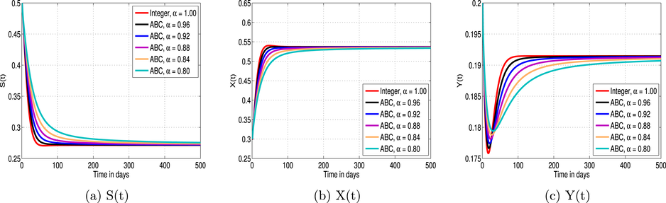
Dynamics of the populations of heroin model at heroin persistence state at different values of α .

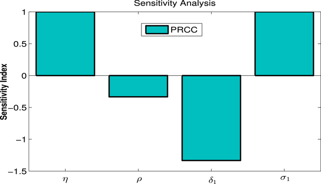
PRCC statistics regarding the significance of factors associated with R 0 .

5.1

5.1 Sensitivity analysis

Making decisions about effectively managing a disease necessitates careful consideration of the sensitivity analysis concept. The sensitivity analysis enables us to examine how variables fluctuate when the parameters in $R_{0}$ are altered. It highlights the model’s most sensitive and impactful parameters and their effects on $R_{0}$ (Butt et al., 2023a,b).

Definition 3

(Butt et al., 2023b) The normalized forward sensitivity index ( $Υ_{ς}$ ) of the basic reproduction number $R_{0}$ that depends on a parameter $ς$ is provided below as:

(71)

Υ_{ς} = \frac{ς}{R_{0}} \frac{\partial R_{0}}{\partial ς} .

To examine the sensitivity of $R_{0}$ , we compute its derivatives as follows: $\frac{\partial R_{0}}{\partial δ_{1}} = - \frac{σ_{1} η (ρ + 2 δ_{1})}{{[δ_{1} (ρ + δ_{1})]}^{2}},$ $\frac{\partial R_{0}}{\partial η} = \frac{σ_{1}}{δ_{1} (ρ + δ_{1})},$ $\frac{\partial R_{0}}{\partial ρ} = - \frac{σ_{1} η}{δ_{1} {(ρ + δ_{1})}^{2}},$ $\frac{\partial R_{0}}{\partial σ_{1}} = \frac{η}{δ_{1} (ρ + δ_{1})} .$ The normalized sensitivity indices of the involved parameters are obtained as: $Υ_{δ_{1}} = \frac{δ_{1}}{R_{0}} \frac{\partial R_{0}}{\partial δ_{1}} = - \frac{2 δ_{1}}{ρ + δ_{1}}, Υ_{η} = \frac{η}{R_{0}} \frac{\partial R_{0}}{η} = 1,$ $Υ_{ρ} = \frac{ρ}{R_{0}} \frac{\partial R_{0}}{ρ} = - \frac{ρ}{ρ + δ_{1}}, Υ_{σ_{1}} = \frac{σ_{1}}{R_{0}} \frac{\partial R_{0}}{\partial σ_{1}} = 1 .$

Table 2 and Fig. 3 depict the favorable influence of $η$ and $σ_{1}$ on the threshold parameter $R_{0}$ . This indicates that higher values of these parameters result in an increase in $R_{0}$ . The sensitivity indices obtained clearly show 10% rise in the new drug users, and infection rate occurs to raise the value of $R_{0}$ by 10%, 10%, correspondingly, and can ultimately leading to a disease outbreak. Across the other perspective, $R_{0}$ is negatively impacted by $δ_{1}$ and $ρ$ as shown by Fig. 4 (see Table 3).

Table 2 Sensitivity indices of

R_{0}

against the parameters.

Sensitivity index	Value
$Υ_{δ_{1}}$	−1.3333
$Υ_{η}$	$+ 1.0000$
$Υ_{ρ}$	−0.3333
$Υ_{σ_{1}}$	$+ 1.0000$

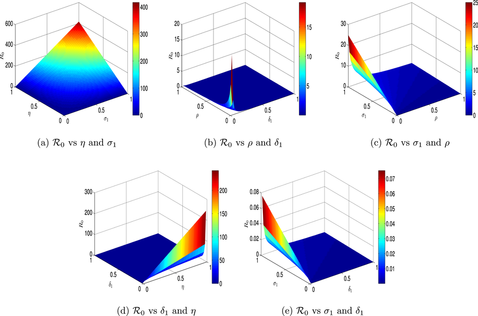
The behaviors of R 0 under different biological parameters.

Table 3 Initial conditions and parameter values of the heroin model.

Initial condition	Value	Source
$S (0)$	0.50	Raza et al. (2022a)
$X (0)$	0.30	Raza et al. (2022a)
$Y (0)$	0.20	Raza et al. (2022a)
Parameter	Value	Source
$η$	0.04	Raza et al. (2022a)
$σ_{1}$	0.02 for $H_{0}$ (0.20 for $H_{1}$ )	Raza et al. (2022a)
$σ_{2}$	0.03	Raza et al. (2022a)
$δ_{1}$	0.04	Raza et al. (2022a)
$ρ$	0.02	Raza et al. (2022a)

5.2

5.2 Numerical results and discussion

This subsection examines the effect of the fractional parameter $α$ on the heroin epidemic disease in the model. A graphical outcome of the model application (8) that depicts the impacts of fractional order on the population in every section. We have illustrated the heroin dynamics of a model for $α = 0.80, 0.84, 0.88, 0.92, 0.96$ and $1$ , respectively. For the heroin-free equilibrium, an elevation in the value of $α$ from 0.80 corresponds to boost in the count of susceptible cases. However, the populations of drug users and non-drug users decline undeviatingly by increasing the value of $α$ from 0.8. In contrast, the susceptible decreases with the rise of fractional parameters in heroin persistence point and the behavior of drug users and non-drug users is observed oppositely, as illustrated by Fig. 2. At the end, when contemplating the case where $α = 1$ , we arrived at the results of Raza et al. (2022a), where a different numerical approach was used. The behavior of the individuals is illustrated in Fig. 5 at different values of $σ_{1}$ by fixing the value of the fractional parameter. These results show a distinct trend, the proportion of susceptible people declines as the infection probability rate rises. The reason for this is that a greater number of people who were previously susceptible to infection are now either recovering or current drug users due to the increased likelihood of infection. On the other hand, as the probability of infection increases, so does the population of drug users. As there is a direct association between the probability of infection and the number of new drug users, this increase happens because a greater infection rate makes more susceptible people more likely to start using drugs. On the other side, the findings indicate a rise in non-drug users, which may be people who have abstained from drug use in the past but have recovered or those who have rejected using drugs despite the risk of infection. The fact that this group is expanding suggests that, despite greater dangers, some members of the population at risk can recover or avoid infection.

The behavior of the individuals is illustrated in Fig. 6 at different values of $σ_{2}$ by fixing the value of the fractional parameter. According to the analysis, fewer people are susceptible to heroin use when the chance rate, that is, the rate at which people are exposed to or attracted by the drug—increases. This occurs because there is a greater probability that those at risk will become drug users when the chance rate is higher. With a rise in the chance rate, there is a consistent rise in the population of drug users. This pattern shows that increasing exposure or temptation rates leads to more people shifting from being vulnerable to actually using heroin. As the chance rate rises, the proportion of non-drug users falls. This group comprises people who have either never used heroin or who have overcome their addiction. This group may decline as a result of a higher chance rate, making it more difficult for people to prevent or rehabilitate from habit.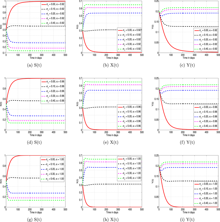

Effect of σ 1 on the behavior of heroin model populations for α = 0 . 92 , 0 . 96 and 1 .

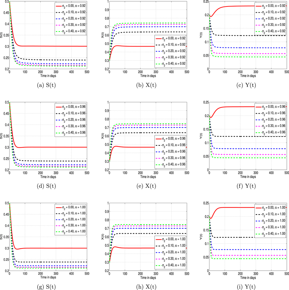
Effect of σ 2 on the behavior of heroin model populations for α = 0 . 96 , 0 . 98 and 1.00.

After examining, it can be stated that the mechanisms of heroin addiction are shaped by both the infection probability rate and the chance rate. A multimodal strategy that incorporates lowering risk factors, improving recovery guides, and putting in place powerful educational activities is necessary for successful management and safeguarding against heroin addiction. Public health measures can more successfully stop the rapid growth of heroin addiction and assist those who are impacted in a successful recovery by considering these factors.

6 Conclusion

In this manuscript, we have developed a novel fractional epidemic model of heroin population consequences by applying the Atangana–Baleanu fractional derivative. The fundamental reproduction number has been determined to investigate the dynamical behavior of the fractional model. The effects of heroin can be controlled by using a reproduction number. The primary properties such as positiveness, boundedness, existence, and uniqueness of the solution have been validated. It has been concluded that the equilibrium states are locally and globally asymptotically stable. In the end, we have applied a computational approach that assesses the dynamics of the proposed system. The results of the numerical technique show that the susceptible people increase with the increase in fractional order, and the other two subpopulations show opposite behavior.

CRediT authorship contribution statement

Miguel Vivas-Cortez: Data curation, Funding acquisition, Methodology. Abu Bakar: Formal analysis, Software, Validation. M.S. Alqarni: Conceptualization, Resource Management, Methodology. Nauman Raza: Investigation,Supervision, Validation. Talat Nazir: Supervision, Project administration, Data curation. Muhammad Farman: Methodology, Validation.

Acknowledgments

The authors extend their appreciation to the Deanship of Research and Graduate Studies at King Khalid University, Saudi Arabia for funding this work through Large Research Project under grant number RGP2/113/45. The authors thank the anonymous referees for their valuable constructive comments and suggestions, which improved the quality of this paper in the present form.

Declaration of competing interest

The authors declare that there is no conflict of interest regarding the submission of this paper.

References

Abdeljawad T., Baleanu D., . Integration by parts and its applications of a new nonlocal fractional derivative with Mittag-Leffler nonsingular kernel. J. Nonlinear Sci.. 2017;10(3):1098-1107.
[CrossRef] [Google Scholar]
Aggarwal G., Uddin I., Şahin A., . On common fixed points of non-Lipschitzian semigroups in a hyperbolic metric space endowed with a graph. J. Anal. 2023:2023.
[CrossRef] [Google Scholar]
Ahmad W., . Mathematical analysis for the effect of voluntary vaccination on the propagation of Corona virus pandemic. Results Phys.. 2021;31:104917
[CrossRef] [Google Scholar]
Ain Qura Tul, . A stochastic approach for co-evolution process of virus and human immune system. Sci. Rep.. 2024;14(1):10337.
[Google Scholar]
Banach S., . Sur les opérations dans les ensembles abstraits et leur application aux équations intégrales. Fund. Math.. 1922;3:133-181.
[Google Scholar]
Bas E., Ozarslan R., . Real world applications of fractional models by Atangana - Aleanu fractional derivative. Chaos Solit. Fractals. 2018;116(2018):121-125.
[CrossRef] [Google Scholar]
Butt A.I.K., . Numerical analysis of Atangana-Baleanu fractional model to understand the propagation of a novel Corona virus pandemic. Alex. Eng. J.. 2022;61(9):7007-7027.
[CrossRef] [Google Scholar]
Butt A.R., . Dynamical analysis of a nonlinear fractional cervical cancer epidemic model with the nonstandard finite difference method. Ain Shams Eng. J. 2023102479
[CrossRef] [Google Scholar]
Butt A.R., . Investigating the fractional dynamics and sensitivity of an epidemic model with nonlinear convex rate. Results Phys.. 2023;54:107089
[CrossRef] [Google Scholar]
Butt A.I.K., . Optimally analyzed fractional coronavirus model with Atangana-Baleanu derivative. Results Phys.. 2023;53:106929
[CrossRef] [Google Scholar]
Chou T., D’Orsogna M.R., . A mathematical model of reward-mediated learning in drug addiction. Chaos. 2022;32(2):021102
[CrossRef] [Google Scholar]
Fabien M., . United nations office on drugs and crime: World drug report 2017. SIRIUS-Zeitschrift für Strategische Analysen. 2018;2(1):85-86.
[Google Scholar]
Glicksberg L., Dempsey S.K., Casey B.K., . Heroin and fentanyl in dallas county: A 5-year retrospective review of toxicological, seized drug, and demographical data. J. Forensic Sci.. 2023;68(1):222-232.
[CrossRef] [Google Scholar]
Gomez-Aguilar J.F., . Atangana-Baleanu fractional derivative applied to electromagnetic waves in dielectric media. J. Electromagn. Waves Appl.. 2016;30(15):1937-1952.
[CrossRef] [Google Scholar]
Huang G., Liu A., . A note on global stability for a heroin epidemic model with distributed delay. Appl. Math. Lett.. 2013;26(7):687-691.
[CrossRef] [Google Scholar]
Khan A., . Optimal control strategies for a heroin epidemic model with age-dependent susceptibility and recovery-age. AIMS Math.. 2021;6(2):1377-1394.
[CrossRef] [Google Scholar]
Lassalle J.P., . The Stability of Dynamical Systems, Regional Conference Series in Applied Mathematics. Philadelphia, Pa, USA: SIAM; 1976.
[CrossRef]
Liu X., Wang L., . Epidemic dynamics on a delayed multi-group heroin epidemic model with nonlinear incidence rate. J. Nonlinear Sci. Appl.. 2016;9(5):2149-2160.
[CrossRef] [Google Scholar]
Mekkaoui T., Atangana A., . New numerical approximation of fractional derivative with non-local and non-singular kernel: Application to chaotic models. Eur. Phys. J. Plus. 2017;132(444):1-16.
[CrossRef] [Google Scholar]
Owolabi K.M., Atangana A., . On the formulation of Adams–Bashforth scheme with Atangana-Baleanu-Caputo fractional derivative to model chaotic problems. Chaos. 2019;29:023111
[CrossRef] [Google Scholar]
Panda S.K., . Applying fixed point methods and fractional operators in the modelling of novel Coronavirus 2019-nCoV/SARS-CoV-2. Results Phys.. 2020;19:103433
[CrossRef] [Google Scholar]
Rashid Saima, . New numerical dynamics of the heroin epidemic model using a fractional derivative with Mittag-Leffler kernel and consequences for control mechanisms. Results Phys.. 2022;35:105304
[Google Scholar]
Raza A., . Dynamical and nonstandard computational analysis of heroin epidemic model. Results Phys.. 2022;34:105245
[CrossRef] [Google Scholar]
Raza N., . Numerical simulations of the fractional-order SIQ mathematical model of Corona virus disease using the nonstandard finite difference scheme. Malays. J. Math. Sci.. 2022;16(3)
[CrossRef] [Google Scholar]
Raza N., . A numerical efficient splitting method for the solution of HIV time periodic reaction–diffusion model having spatial heterogeneity. Phys. A. 2023;609:128385
[CrossRef] [Google Scholar]
Riaz Muhammad Bilal, . Fractional dynamics and sensitivity analysis of measles epidemic model through vaccination. Arab J. Basic Appl. Sci.. 2024;31(1):265-281.
[Google Scholar]
Saha S., Samanta G.P., . Dynamics of an epidemic model with impact of toxins. Phys. A. 2019;527:121152
[CrossRef] [Google Scholar]
Şahin A., Alagöz O., . On the approximation of fixed points for the class of mappings satisfying (CSC)-condition in Hadamard spaces. Carpathian Math. Publ.. 2023;15(2):495-506.
[CrossRef] [Google Scholar]
Şahin A., Öztürk E., Aggarwal G., . Some fixed-point results for the $K F$ -iteration process in hyperbolic metric spaces. Symmetry. 2023;15(7):1360.
[CrossRef] [Google Scholar]
Syam M.I., Al-Refai M., . Fractional differential equations with Atangana-Baleanu fractional derivative: Analysis and applications. Chaos Solit. Fractals X. 2019;2:100013
[CrossRef] [Google Scholar]
Tolomeo S., Steele J.D., Ekhtiari H., Alex B., . Chronic heroin use disorder and the brain: Current evidence and future implications. Progr. Neuro-Psychopharmacol. Biol. Psychiat.. 2021;111:110148
[CrossRef] [Google Scholar]
Wangari I.M., Stone L., . Analysis of a heroin epidemic model with saturated treatment function. J. Appl. Math. (2017)
[CrossRef] [Google Scholar]
Weera W., . A neural study of the fractional heroin epidemic model. Comput. Mater. Contin.. 2023;74(2):2.
[CrossRef] [Google Scholar]
Xu J., . Dynamical analysis of a heroin - cocaine epidemic model with nonlinear incidence and spatial heterogeneity. J. Biol. Dyn.. 2023;17(1):2189026
[CrossRef] [Google Scholar]
Zafar Z.U.A., . Fractional order heroin epidemic dynamics. Alex. Eng. J.. 2021;60(6):5157-5165.
[CrossRef] [Google Scholar]
Zhang L., Xing Y., . Stability analysis of a reaction–diffusion heroin epidemic model. Complexity 2020:1-16.
[CrossRef] [Google Scholar]

Data availability

Introduction

Formulation and configuration of heroin model

Existence and uniqueness of heroin model

Qualitative perspectives of the heroin model

Equilibrium points and basic reproduction number
Stability analysis

Numerical analysis

Sensitivity analysis
Numerical results and discussion

Conclusion

CRediT authorship contribution statement

Fulltext Views
6

PDF downloads
2

View/Download PDF
Download Citations

BibTeX
RIS

Show Sections

[1] Abdeljawad T., Baleanu D., . Integration by parts and its applications of a new nonlocal fractional derivative with Mittag-Leffler nonsingular kernel. J. Nonlinear Sci.. 2017;10(3):1098-1107.
[CrossRef] [Google Scholar]

[2] Aggarwal G., Uddin I., Şahin A., . On common fixed points of non-Lipschitzian semigroups in a hyperbolic metric space endowed with a graph. J. Anal. 2023:2023.
[CrossRef] [Google Scholar]

[3] Ahmad W., . Mathematical analysis for the effect of voluntary vaccination on the propagation of Corona virus pandemic. Results Phys.. 2021;31:104917
[CrossRef] [Google Scholar]

[4] Ain Qura Tul, . A stochastic approach for co-evolution process of virus and human immune system. Sci. Rep.. 2024;14(1):10337.
[Google Scholar]

[5] Banach S., . Sur les opérations dans les ensembles abstraits et leur application aux équations intégrales. Fund. Math.. 1922;3:133-181.
[Google Scholar]

[6] Bas E., Ozarslan R., . Real world applications of fractional models by Atangana - Aleanu fractional derivative. Chaos Solit. Fractals. 2018;116(2018):121-125.
[CrossRef] [Google Scholar]

[7] Butt A.I.K., . Numerical analysis of Atangana-Baleanu fractional model to understand the propagation of a novel Corona virus pandemic. Alex. Eng. J.. 2022;61(9):7007-7027.
[CrossRef] [Google Scholar]

[8] Butt A.R., . Dynamical analysis of a nonlinear fractional cervical cancer epidemic model with the nonstandard finite difference method. Ain Shams Eng. J. 2023102479
[CrossRef] [Google Scholar]

[9] Butt A.R., . Investigating the fractional dynamics and sensitivity of an epidemic model with nonlinear convex rate. Results Phys.. 2023;54:107089
[CrossRef] [Google Scholar]

[10] Butt A.I.K., . Optimally analyzed fractional coronavirus model with Atangana-Baleanu derivative. Results Phys.. 2023;53:106929
[CrossRef] [Google Scholar]

[11] Chou T., D’Orsogna M.R., . A mathematical model of reward-mediated learning in drug addiction. Chaos. 2022;32(2):021102
[CrossRef] [Google Scholar]

[12] Fabien M., . United nations office on drugs and crime: World drug report 2017. SIRIUS-Zeitschrift für Strategische Analysen. 2018;2(1):85-86.
[Google Scholar]

[13] Glicksberg L., Dempsey S.K., Casey B.K., . Heroin and fentanyl in dallas county: A 5-year retrospective review of toxicological, seized drug, and demographical data. J. Forensic Sci.. 2023;68(1):222-232.
[CrossRef] [Google Scholar]

[14] Gomez-Aguilar J.F., . Atangana-Baleanu fractional derivative applied to electromagnetic waves in dielectric media. J. Electromagn. Waves Appl.. 2016;30(15):1937-1952.
[CrossRef] [Google Scholar]

[15] Huang G., Liu A., . A note on global stability for a heroin epidemic model with distributed delay. Appl. Math. Lett.. 2013;26(7):687-691.
[CrossRef] [Google Scholar]

[16] Khan A., . Optimal control strategies for a heroin epidemic model with age-dependent susceptibility and recovery-age. AIMS Math.. 2021;6(2):1377-1394.
[CrossRef] [Google Scholar]

[17] Lassalle J.P., . The Stability of Dynamical Systems, Regional Conference Series in Applied Mathematics. Philadelphia, Pa, USA: SIAM; 1976.
[CrossRef]

[18] Liu X., Wang L., . Epidemic dynamics on a delayed multi-group heroin epidemic model with nonlinear incidence rate. J. Nonlinear Sci. Appl.. 2016;9(5):2149-2160.
[CrossRef] [Google Scholar]

[19] Mekkaoui T., Atangana A., . New numerical approximation of fractional derivative with non-local and non-singular kernel: Application to chaotic models. Eur. Phys. J. Plus. 2017;132(444):1-16.
[CrossRef] [Google Scholar]

[20] Owolabi K.M., Atangana A., . On the formulation of Adams–Bashforth scheme with Atangana-Baleanu-Caputo fractional derivative to model chaotic problems. Chaos. 2019;29:023111
[CrossRef] [Google Scholar]

[21] Panda S.K., . Applying fixed point methods and fractional operators in the modelling of novel Coronavirus 2019-nCoV/SARS-CoV-2. Results Phys.. 2020;19:103433
[CrossRef] [Google Scholar]

[22] Rashid Saima, . New numerical dynamics of the heroin epidemic model using a fractional derivative with Mittag-Leffler kernel and consequences for control mechanisms. Results Phys.. 2022;35:105304
[Google Scholar]

[23] Raza A., . Dynamical and nonstandard computational analysis of heroin epidemic model. Results Phys.. 2022;34:105245
[CrossRef] [Google Scholar]

[24] Raza N., . Numerical simulations of the fractional-order SIQ mathematical model of Corona virus disease using the nonstandard finite difference scheme. Malays. J. Math. Sci.. 2022;16(3)
[CrossRef] [Google Scholar]

[25] Raza N., . A numerical efficient splitting method for the solution of HIV time periodic reaction–diffusion model having spatial heterogeneity. Phys. A. 2023;609:128385
[CrossRef] [Google Scholar]

[26] Riaz Muhammad Bilal, . Fractional dynamics and sensitivity analysis of measles epidemic model through vaccination. Arab J. Basic Appl. Sci.. 2024;31(1):265-281.
[Google Scholar]

[27] Saha S., Samanta G.P., . Dynamics of an epidemic model with impact of toxins. Phys. A. 2019;527:121152
[CrossRef] [Google Scholar]

[28] Şahin A., Alagöz O., . On the approximation of fixed points for the class of mappings satisfying (CSC)-condition in Hadamard spaces. Carpathian Math. Publ.. 2023;15(2):495-506.
[CrossRef] [Google Scholar]

[29] Şahin A., Öztürk E., Aggarwal G., . Some fixed-point results for the $K F$ -iteration process in hyperbolic metric spaces. Symmetry. 2023;15(7):1360.
[CrossRef] [Google Scholar]

[30] Syam M.I., Al-Refai M., . Fractional differential equations with Atangana-Baleanu fractional derivative: Analysis and applications. Chaos Solit. Fractals X. 2019;2:100013
[CrossRef] [Google Scholar]

[31] Tolomeo S., Steele J.D., Ekhtiari H., Alex B., . Chronic heroin use disorder and the brain: Current evidence and future implications. Progr. Neuro-Psychopharmacol. Biol. Psychiat.. 2021;111:110148
[CrossRef] [Google Scholar]

[32] Wangari I.M., Stone L., . Analysis of a heroin epidemic model with saturated treatment function. J. Appl. Math. (2017)
[CrossRef] [Google Scholar]

[33] Weera W., . A neural study of the fractional heroin epidemic model. Comput. Mater. Contin.. 2023;74(2):2.
[CrossRef] [Google Scholar]

[34] Xu J., . Dynamical analysis of a heroin - cocaine epidemic model with nonlinear incidence and spatial heterogeneity. J. Biol. Dyn.. 2023;17(1):2189026
[CrossRef] [Google Scholar]

[35] Zafar Z.U.A., . Fractional order heroin epidemic dynamics. Alex. Eng. J.. 2021;60(6):5157-5165.
[CrossRef] [Google Scholar]

[36] Zhang L., Xing Y., . Stability analysis of a reaction–diffusion heroin epidemic model. Complexity 2020:1-16.
[CrossRef] [Google Scholar]

Global stability and modeling with a non-singular kernel for fractional order heroin epidemic model: Insights from different population studies

Abstract

Keywords

Heroin epidemic model

Atangana–Baleanu fractional derivative

Sensitivity analysis

Stability

Numerical solution

Data availability

1 Introduction

2 Formulation and configuration of heroin model

3 Existence and uniqueness of heroin model

Theorem 1 Banach, 1922

4 Qualitative perspectives of the heroin model

4.1 Equilibrium points and basic reproduction number

4.2 Stability analysis

4.2.1 Stability of heroin free equilibrium point H 0

Theorem 5 Butt et al., 2023a

Theorem 6 Butt et al., 2023a

4.2.2 Stability of heroin persistence equilibrium point H 1

Theorem 7 Butt et al., 2023a

Theorem 8 Butt et al., 2023a

5 Numerical analysis

5.1 Sensitivity analysis

5.2 Numerical results and discussion

6 Conclusion

CRediT authorship contribution statement

Acknowledgments

Declaration of competing interest

References

Suggested read for related articles:

4.2.1 Stability of heroin free equilibrium point $H_{0}$

4.2.2 Stability of heroin persistence equilibrium point $H_{1}$