

Jacobi elliptic function solutions for a two-mode KdV equation
⁎Corresponding author. marwan04@just.edu.jo (Marwan Alquran)
-
Received: ,
Accepted: ,
This article was originally published by Elsevier and was migrated to Scientific Scholar after the change of Publisher.
Peer review under responsibility of King Saud University.
Abstract
In this paper we introduce a new type of KdV equations called Two-mode KdV (TMKdV). This equation represents the propagation of two-wave modes in the same direction simultaneously. We suggest a finite series of degree n in terms of a Jacobi elliptic functions as a possible solution for the TMKdV. We succeeded in obtaining new solutions of type solitons and periodics.
Keywords
Jacobi elliptic function methods
Two-mode KdV equation
35C08
74J35

1 Introduction
Most of nonlinear equations are defined by first-order partial differential equation (PDE) in time. They describe unidirectional waves where these equations model one right-moving for
The TMKdV Eq. (1.1) was studied recently in the literature. Analytic methods for this equation have been used, such as the reductive perturbation (Lee and Liu, 2011), Hamiltonian system (Lee and Lee, 2013), Bell polynomials (Hong and Jung, 1999), and others. In Xiao et al. (2016), it was found that both the two solitons in the two modes separate without any change of their initial shapes and velocities except for the phase shifts after each collision. In Lee et al. (2010), three basic conserved quantities, namely, the mass, momentum, and Hamiltonian for the TMKdV equation were constructed by using the prolongation method.
Many models in mathematics and physics are described by nonlinear partial differential equations (NPDEs). The theory of solitary wave solution has contributed to understanding many experiments and complex phenomena in mathematical physics. Thus, the literature has been enriched by well imposed methods that produce exact solutions of such nonlinear equations. Such methods are: The sine-cosine method (Wazwaz, 2004; Alquran and Qawasmeh, 2013; Alquran, 2012), Rational sine-cosine (Qawasmeh and Alquran, 2014), tanh method (Alquran and Al-Khaled, 2011), extended tanh method (Shukri and Al-khaled, 2010), sech-tanh method (Alquran et al., 2012), Exp-function method (Raslan, 2009), the
The goal of this work is to explore more new exact solutions of the two-mode KdV equation given in (1.1) by using a finite series of degree n in terms of a Jacobi elliptic functions (Liu et al., 2001; Fu et al., 2001) which belongs to the well-known homogeneous balance principle and truncated function expansion method (Fan and Zhang, 1998, 2002; Dai and Zhang, 2006; Liu et al., 2001).
2 Jacobi elliptic sine and cosine functions
In this section we introduce in details the derivation of Jacobi elliptic functions. First, we consider the second order partial deferential equation (PDE)
Applying the linear transformation
By forcing
Separating the variables in (2.5) leads to the following integral
Now, we define
Therefore,
Thus, we reach to the identities,
Thus,
Now we are ready ti introduce the following formulas
Also, we can observe by the second equation of (2.13) that,
Therefore,
Equivalently,
Thus,
Also,
Now, if
Figs. 1 and 2 represent the functions
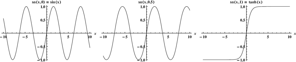
- Plots of the Jacobi
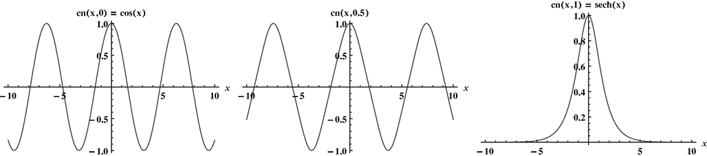
- Plots of the Jacobi
Now, we will highlight briefly the main steps of the Jacobi elliptic sine-cosine expansion method. We first unite the independent variables x and t into one wave variable
Eq. (2.21) is then integrated as long as all terms contain derivatives. The Jacobi elliptic sine-cosine technique is based on the assumption that the traveling wave solutions can be expressed in terms of the
Then, the solution can be proposed a finite power series in Y in the form:
The parameter M is a positive integer, in most cases, that will be determined by using a balance procedure, where by comparing the behavior of
3 Solutions of the two-mode KdV equation
In this section, we apply the Jacobi elliptic sine-cosine expansion method to extract possible solutions of (1.1). By using the wave variable
To determine the coefficients
Some of the equation in the above system have been deleted where
Therefore, the Jacobi sine solution of the two-mode KdV equation is
If
Now we proceed as above but replacing the Jacobi sine by Jacobi cosine function in (3.2), i.e.,
Following the procedures considered as in the Jacobi Sine case, one can reach to the following results
Therefore, the Jacobi cosine solution of the two-mode KdV equation is
If
Finally, if we use the Jacobi DN Solution to the two-mode KdV equation, we get the same obtained solution as given in (3.9) but with value of
4 Discussion and concluding remarks
In this work, we succeeded in obtaining Jacobi elliptic sine-cosine solutions for the proposed two-mode KdV Eq. (1.1). We may reduce the calculations performed in the previous section and obtain the Jacobi cosine solution given in (3.9) by using the identity
The types of the obtained solutions given in (3.6) and (3.10) are solitons. Solitons are solutions in the form sech and
By using the facts
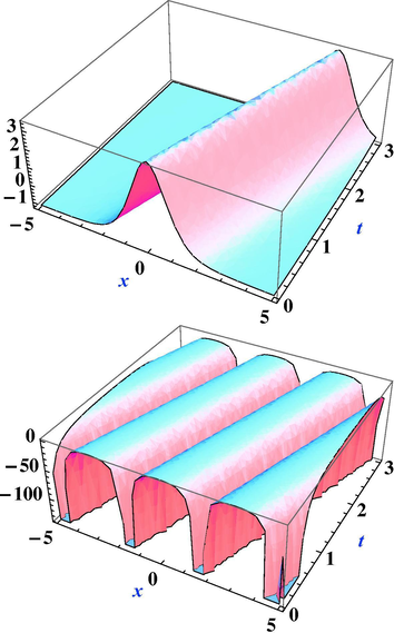
- The obtained solutions of the TMKdV given in (3.6) and (4.1) respectively when
References
- Solitons and periodic solutions to nonlinear partial differential equations by the Sine-Cosine method. Appl. Math. Inf. Sci.. 2012;6(1):85-88.
- [Google Scholar]
- The tanh and sine-cosine methods for higher order equations of Korteweg-de Vries type. Phys. Scr..
- Classifications of solutions to some generalized nonlinear evolution equations and systems by the sine-cosine method. Nonlinear Stud.. 2013;20(2):263-272.
- [Google Scholar]
- Soliton solutions of shallow water wave equations by means of
- [Google Scholar]
- Solitary wave solutions to shallow water waves arising in fluid dynamics. Nonlinear Stud.. 2012;19(4):555-562.
- [Google Scholar]
- Jacobian elliptic function method for nonlinear differential-difference equations. Chaos, Solitons Fractals. 2006;27:1042-1049.
- [Google Scholar]
- Applications of the Jacobi elliptic function method to special-type nonlinear equations. Phys. Lett A. 2002;305:383-392.
- [Google Scholar]
- New Jacobi elliptic function expansion and new periodic solutions of nonlinear wave equations. Phys. Lett. A. 2001;290:72-76.
- [Google Scholar]
- Variational method for the derivative nonlinear Schrodinger equation with computational applications. Phys. Scr.. 2009;80(3):350-360.
- [Google Scholar]
- New non-traveling solitary wave solutions for a second-order Korteweg-de Vries equation. Z. Naturforsch.. 1999;54a:375-378.
- [Google Scholar]
- Soliton solutions for a second-order KdV equation. Phys. Lett. A. 1994;185:174-176.
- [Google Scholar]
- On wave solutions of a weakly nonlinear and weakly dispersive two-mode wave system. Waves Random Complex Medium. 2013;23:56-76.
- [Google Scholar]
- A Hamiltonian model and soliton phenomenon for a two-mode KdV equation, Rocky Mountain. J. Math.. 2011;41(4):1273-1289.
- [Google Scholar]
- Quasi-solitons of the two-mode Korteweg-de Vries equation. Eur. Phys. J. Appl. Phys.. 2010;52:11-301.
- [Google Scholar]
- Jacobi elliptic function expansion method and periodic wave solutions of nonlinear wave equations. Phys. Lett. A. 2001;289:69-74.
- [Google Scholar]
- Jacobi elliptic function expansion method and periodic wave solutions of nonlinear wave equations. Phys. Lett. A. 2001;289(1–2):69-74.
- [Google Scholar]
- Reliable study of some new fifth-order nonlinear equations by means of
- [Google Scholar]
- Soliton and periodic solutions for
- [Google Scholar]
- The application of Hes Exp-function method for MKdV and Burgers equations with variable coefficients. Int. J. Nonlinear Sci.. 2009;7(2):174-181.
- [Google Scholar]
- Stability analysis for Zakharov-Kuznetsov equation of weakly nonlinear ion-acoustic waves in a plasma. Comp. Math. Appl.. 2014;67:172-180.
- [Google Scholar]
- Fractional solitary wave solutions of the nonlinear higher-order extended KdV equation in a stratified shear flow: part I. Comp. Math. Appl.. 2015;70:345-352.
- [Google Scholar]
- Stability analysis solutions for nonlinear three-dimensional modified Korteweg-de Vries-Zakharov-Kuznetsov equation in a magnetized electron-positron plasma. Phys. A. 2016;455:44-51.
- [Google Scholar]
- Travelling-wave solutions of a weakly nonlinear two-dimensional higher-order Kadomtsev-Petviashvili dynamical equation for dispersive shallow-water waves. Eur. Phys. J. Plus. 2017;132:29.
- [Google Scholar]
- Traveling wave solutions for some coupled nonlinear evolution equations. Math. Comput. Modell.. 2013;57(5):1371-1379.
- [Google Scholar]
- The extended tanh method for solving systems of nonlinear wave equations. Appl. Math. Comput.. 2010;217(5):1997-2006.
- [Google Scholar]
- A sine-cosine method for handling nonlinear wave equations. Math. Comput. Modell.. 2004;40(5–6):499-508.
- [Google Scholar]
- Multi-soliton solutions and Bäcklund transformation for a two-mode KdV equation in a fluid. Waves Random Complex Medium. 2016;31(6):1-4.
- [Google Scholar]
- Solitary wave solutions having two wave modes of KdV-type and KdV-burgers-type. Chin. J. Phys.. 1997;35(6):633-639.
- [Google Scholar]


