An efficient modification of the decomposition method with a convergence parameter for solving Korteweg de Vries equations

1 Introduction

The well-known evolution equations that occur frequently in mathematical physics and shallow water applications can be formulated as

where $f\left(x,t\right)$ is the homogeneous term function; $C,a_m$ , $b_m$ real constants; $k$ and $i$ natural numbers and $M\mathrm{a}\mathrm{n}\mathrm{d}N$ are nonnegative integers. The exact solution of Eq. (1) is always very difficult to find (Yusuf et al., 2018) which necessitates the study of its special cases including the Korteweg de Vries (KdV) equation, the Benjamin–Bona–Mahony equation (BBM), the Burger’s equation and the regularized long-wave equation (RLWE) among others. The well-known KdV equation reads

where $r$ is a constant mostly preferred 1 or 6 for solution description, see (Soliman and Abdou, 2008; Syam, 2005; Varley and Seymour, 1998; Wazwaz, 1999; Wazwaz, 2001). Recently, the Adomian decomposition method (ADM) (Adomian, 1983; Adomian, 1986; Adomian, 1988; Adomian, 1991; Adomian and Rach, 1992) has been broadly used in treating a variety of mathematical problems mostly modeled in nonlinear differential and integral equations (Aly et al., 2012; AlQarni et al., 2016; Bakodah, 2012; Bakodah, 2012; Bakodah et al., 2017; Bakodah et al., 2015; Bakodah and Darwish, 2013; Bakodah et al., 2016; Banaja et al., 2017; Bulut et al., 2013); see also (Sabi'u et al., 2018; Ebaid, 2011; Ebaid et al., 2015; Duan and Rach, 2011; Duan et al., 2012; Duan, 2010; Inc et al., 2018; Nuruddeen et al., 2018; Qureshi and Ramos, 2018) for various modifications of the ADM and (Liao, 2010; Rach, 1987; Schiesser, 1994; Abdel-Gawad et al., 2018; Aliya et al., 2018; Ansari et al., 2018; Yusuf et al., 2018; Zhang and Liang, 2016) for other methods for solving various evolution equations, respectively. The main part of the ADM is generating the Adomian's polynomials

with $A_n$ denoting the Adomian's polynomials of degree $n$ for the nonlinear term appearing in the considered equation while $u={\sum }_{i=0}^{\infty }{u}_i(x,t)$ is the series solution converging to the exact one. Furthermore, in the case of the Adomian's polynomials for multivariable nonlinearities and differential nonlinearities, we have $$A_n=\frac{1}{n!}{\left[\frac{d^n}{d{\lambda }^n}N\left(\sum _{i=0}^n{\lambda }^i{u}_{1,i},\cdots ,\sum _{i=0}^n{\lambda }^i{u}_{m,i}\right)\right]}_{\lambda =0},n\ge 0,$$

where $N\left(u_1,\cdots ,u_m\right)$ is the multivariable nonlinearity of $m$ arguments. Again, both the one and multivariable Adomian’s polynomials can respectively be rapidly generated to high orders by algorithms and Mathematica subroutines crafted by Duan (Inc et al., 2018). Moreover, Zhang and Liang (2016) recently proposed a new convergence parameter for the ADM that controls the convergence-region and the rate of the optimal series solution. However, the recent modification of the ADM based on Zhang and Liang (2016) will be proposed in this paper for a class of evolution equations, particularly the KdV equations. Some special test problems of interest would be numerically analyzed by the proposed scheme and provide the error estimate and analysis. The extension of the domain of convergence which provides more accurate approximations can be regarded as the main advantage of the scheme.

2 Analysis of the standard ADM

Considering the linear operators $$L_{x^m}=\frac{{\partial }^m}{{\partial x}^m}\mathrm{a}\mathrm{n}\mathrm{d}{L}_t=\frac{\partial }{\partial t};$$

Eq. (1) can be expressed as

with $L_t^{-1}\left(.\right)={\int }_0^t\left(.\right)dt$ as the inversion operator of $L_t.$

Applying the above inversion operator coupled to initial data $u\left(x,0\right)=h\left(x\right)$ $\mathrm{o}\mathrm{n}$ Eq. (4), we obtain

Thus, the standard ADM offers the following sequential recursion solution of Eq. (1) by decomposing $u\left(x,t\right)$ to infinite series ${\sum }_{n=0}^{\infty }{u}_n\left(x,t\right)$ as $$u_0\left(x,t\right)=h\left(x\right)+L_t^{-1}\left(f\left(x,t\right)\right),$$

where $A_n,n\ge 0$ , are the Adomian polynomials (Adomian, 1983; Adomian, 1986; Adomian, 1988; Adomian, 1991).

3 Analysis of the ADM with a convergence parameter

In this section, the concept of a convergence parameter Zhang and Liang (2016) shall be applied to derive the general recursive scheme of Eq. (1) and later demonstrate its application to solve several special cases in the next section. To begin with, a convergence-control parameter c and an artificial parameter $∊$ are introduced to Eq. (4) which reads

One then set

Applying the inversion operator $L_t^{-1}$ on Eq. (7) $,$ we get

Now, putting Eq. (8) into Eq. (9) and bringing together the coefficients of like-powers of $∊;$ we obtain the following recursive scheme:

with $B_n$ the Adomian's polynomials to be computed using $$B_n=\frac{1}{n!}{\left[\frac{d^n}{d{∊}^n}N\left(\sum _{i=0}^n{∊}^i{v}_i(x,t,c)\right)\right]}_{∊=0},n\ge 0.$$

When $∊$  = 1 in Eq. (8), the solution $u\left(x,t\right)$ with convergence-parameter c is presented by

Then we calculate an n^th-order approximation to the solution as $${\phi }_{m+1}\left(x,t,c\right)=\sum _{n=0}^m{v}_n(x,t,c).$$

To extend the domain of convergence or rather obtain more accurate approximations; the value of the parameter $c$ is to be determined using the discrete averaged square residual error defined as (Nuruddeen et al., 2018)

Further, the averaged residual error $E_m$ against the determined value of $c$ gives the optimal value of $c$ when plotted. We will demonstrate later that the new approach is easily implemented on any symbolic software such as Maple or Mathematica. Also, the optimal value of c is obtained via solving the differential equation $$\frac{\partial E\left(x,t,c\right)}{\partial c}=0.$$

Finally, it can be remarked that the optimal choice of $c$ could significantly be improve the convergence region and rate of the series solution. We show the effectiveness of the present approach by investigating certain test KdV and coupled KdV systems.

4 Applications

The present section demonstrates the high-accuracy of presented method by considering certain KdV and coupled KdV systems of type Eq. (1). We will present the numerical results based on our method and demonstrate its accuracy by studying the absolute error and the number of iterations involved.

Here, $v_0\left(x,0,c\right)$ is selected as $v_0\left(x,t,c\right)=g\left(x,t\right)=\frac{1}{6}\left(x-1\right),$ and consequently Eq. (10) leads to $$v_1\left(x,t,c\right)=c{\int }_0^t[({v_0(x,t,c))}_{3x}-a{B}_0]dt,$$ $$v_2\left(x,t,c\right)=c{\int }_0^t[({v_1(x,t,c))}_{3x}-a{B}_1]dt+\left(1-c\right){\int }_0^t[({v_0(x,t,c))}_{3x}-a{B}_0]dt.$$

Using the parameterized recursion scheme in Eq. (10) with the appropriate Adomian polynomials yields the first several solution components as

and so on. Substituting Eqs. (14)–(17) into Eq. (11) gives the solution $u(x,t)$ , from which it can easily be verified that the closed form solution when $c=0$ is in this form:

Also, to validate the obtained solutions, the curves of the discrete averaged square residual errors $E_m$ versus $c$ are shown in Fig. 1. This figure points out that the optimal value of $c$ is about $1.3392966$ .

Close

Fig. 1

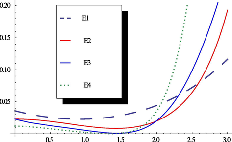
The residual errors at m = 1, 2, 3, 4, and 5.

Export to PPT

The results produced by the proposed method are overall more accurate than the standard ADM, as shown in Table 1a.

The results in Table 1a reveal that the proposed approach is more accurate than the standard ADM in most cases for the chosen values for $x$ and $t$ (Fig. 2).

Close

Fig. 2

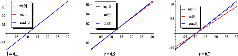
The plots of the exact, proposed method and the ADM solutions, respectively at t = 0.1, 0.5 and 0.7.

Export to PPT

(i) The first version is given by the following equation

with the initial condition

where $a$ is any real constant. On applying the analysis of the previous example, the first several solution components are computed as $$v_0\left(x,t\right)=a-\frac{4a}{1+4a^2{x}^2},$$ $$v_1\left(x,t\right)=-\frac{192a^{5}ctx}{{(1+4a^2{x}^2)}^2},$$ $$v_2\left(x,t\right)=-\frac{192a^{5}t(x-cx+36a^4{c}^{2}t{x}^2+a^2(-3c^{2}t-4(-1+c)x^3))}{{(1+4a^2{x}^2)}^3},$$ $$v_3\left(x,t\right)=-\frac{1}{{\left(1+4a^2{x}^2\right)}^4}1152a^{7}c{t}^2\left(-1+8a^2{x}^2+48a^4{x}^4+48a^4{c}^{2}tx\left(-1+4a^2{x}^2\right)+c\left(1-8a^2{x}^2-48a^4{x}^4\right)\right),$$

and so on. The other calculated terms give the closed form solution when c = 0 as $$u\left(x,t\right)=a-\frac{4a}{(4a^2({x-6a^{2}t)}^2+1)}.$$

Fig. 3 gives the plots of the averaged residual errors $E_m$ against $c$ showing the optimal value of $c$ around 1.001.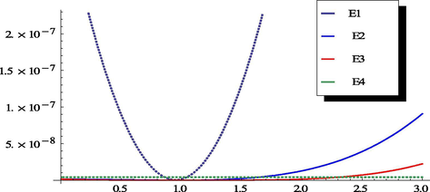

Close

Fig. 3

The residual errors at m = 1, 2, 3, and 4.

Export to PPT

The results produced by our method are put side by side with those obtained by the standard ADM and listed in Table 2. The profile of the solitary wave at $t=0.5$ is displayed in Fig. 4.

Close

Fig. 4

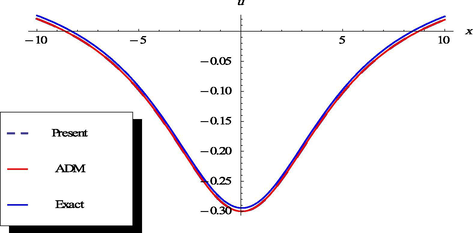
The plots of the exact, proposed method and the ADM solutions, respectively at $t=1.0$ .

Export to PPT

(ii) The second version of the mKdV equation has the traveling wave solution with the initial data:

with $k$ constant and for $a\ge 0$ .

Repeating the previous analysis, we have $$v_0\left(x,t\right)=\sqrt{a}\mathrm{S}\mathrm{e}\mathrm{c}\mathrm{h}(k+\sqrt{a}x),$$ $$v_1\left(x,t\right)=a^{2}ct\mathrm{S}\mathrm{e}\mathrm{c}\mathrm{h}(k+\sqrt{a}x)\mathrm{T}\mathrm{a}\mathrm{n}\mathrm{h}(k+\sqrt{a}x),$$ $$v_2\left(x,t\right)=\frac{1}{4}{a}^{2}t{\mathrm{S}\mathrm{e}\mathrm{c}\mathrm{h}(k+\sqrt{a}x)}^3\left(a^{3/2}{c}^{2}t\left(-3+\mathrm{C}\mathrm{o}\mathrm{s}\mathrm{h}\left[2\left(k+\sqrt{a}x\right)\right]\right)-2\left(-1+c\right)\mathrm{S}\mathrm{i}\mathrm{n}\mathrm{h}\left[2\left(k+\sqrt{a}x\right)\right]\right),$$ $${\mathrm{v}}_3\left(\mathrm{x},\mathrm{t}\right)=\frac{1}{24}{\mathrm{a}}^{7/2}\mathrm{c}{\mathrm{t}}^2{\mathrm{S}\mathrm{e}\mathrm{c}\mathrm{h}(\mathrm{k}+\sqrt{\mathrm{a}}\mathrm{x})}^4\left(30\left(-1+\mathrm{c}\right)\mathrm{C}\mathrm{o}\mathrm{s}\mathrm{h}(\mathrm{k}+\sqrt{\mathrm{a}}\mathrm{x})-6\left(-1+\mathrm{c}\right)\mathrm{C}\mathrm{o}\mathrm{s}\mathrm{h}\left[3\left(\mathrm{k}+\sqrt{\mathrm{a}}\mathrm{x}\right)\right]+{\mathrm{a}}^{3/2}{\mathrm{c}}^2\mathrm{t}\left(-23\mathrm{S}\mathrm{i}\mathrm{n}\mathrm{h}\left[\mathrm{k}+\sqrt{\mathrm{a}}\mathrm{x}\right]+\mathrm{S}\mathrm{i}\mathrm{n}\mathrm{h}\left[3\left(\mathrm{k}+\sqrt{\mathrm{a}}\mathrm{x}\right)\right]\right)\right),$$

and so on. At $c=0,$ the other calculated terms give the following exact solution:

Here also, Fig. 5 gives the plots of the averaged residual errors $E_m$ against $c$ showing the optimal value of $c$ around 1.03.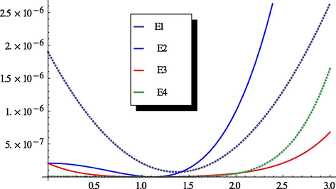

Close

Fig. 5

The residual errors at m = 1, 2, 3, and 4.

Export to PPT

The results derived by the present method are much better than those obtained by the standard ADM as showed in Table 3. In addition, the profile of the solitary wave at time $t=0.5$ is compared in Fig. 6.

Close

Fig. 6

The plots of the exact, proposed method and the ADM solutions, respectively at t = 1.0.

Export to PPT

where $r_1$ and $r_2$ are constants with the following initial data: $$u\left(x,0\right)=\alpha +\gamma \mathrm{csch}(kx),k=\sqrt{\beta },\alpha =-\frac{r_1}{2r_2}\mathrm{a}\mathrm{n}\mathrm{d}\gamma =\sqrt{\frac{6\beta }{r_2}.}$$

We thus obtain the following solitary-wave solution iteratively upon choice of $r_1=1$ , $r_2$  = 1, $\alpha =1\text{and}\beta =0.0001$ as follows: $$u_1\left(x,t\right)=2.449489\times {10}^{-8}ctSech(0.01x)Tanh(0.01x)\left(-2499.99+1.{\mathit{Sech}(0.01x)}^2+0.9999996{\mathit{Tanh}(0.01x)}^2\right),$$ $$u_2\left(x,t\right)=tSech(0.01x)\left(6.123724\times {10}^{-14}{c}^{2}t{\mathit{Sech}(0.01x)}^6-0.000061Tanh(0.01x)+\left(2.44948\times {10}^{-8}-2.44948\times {10}^{-8}c\right){\mathit{Tanh}(0.01x)}^3-3.061862\times {10}^{-11}{c}^{2}t{\mathit{Tanh}(0.01x)}^4+1.2247\times {10}^{-14}{c}^{2}t{\mathit{Tanh}(0.01x)}^6+c^{2}t{\mathit{Sech}(0.01x)}^4\left(-1.530931\times {10}^{-10}-1.592168\times {10}^{-13}{\mathit{Tanh}(0.01x)}^2\right)+{\mathit{Sech}(0.01x)}^{2}Tanh(0.01x)\left(2.44948\times {10}^{-8}+1.2247448\times {10}^{-7}c+5.5113519\times {10}^{-10}{c}^{2}tTanh(0.01x)-2.08206\times {10}^{-13}{c}^{2}t{\mathit{Tanh}(0.01x)}^3\right)\right),$$

and so on. The other calculated terms give the closed form solution as

We illustrate the plots of the residual errors $E_m$ against $c$ with the optimal value of $c$ approaches $0.556$ in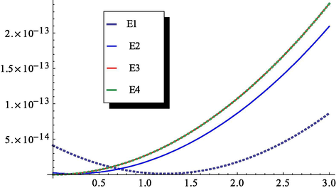 Fig. 7.

Close

Fig. 7

The residual errors at m = 1, 2, 3, and 4.

Export to PPT

The results obtained by the proposed scheme are in good conformity with that of the standard ADM, listed in Table 4. In addition, the profiles of the solitary wave at $t=0.5\mathrm{a}\mathrm{n}\mathrm{d}1.0$ are compared in Figs. 8 and 9.

Close

Fig. 8

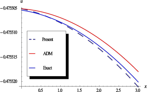
The plots of the exact, proposed method and the ADM solutions, respectively at t = 0.5.

Export to PPT

Close

Fig. 9

The plots of the exact, proposed method and the ADM solutions, respectively at t = 1.0.

Export to PPT

with initial data $$u\left(x,0\right)=\frac{{\mathrm{b}}_1}{2k}+k\mathrm{T}\mathrm{a}\mathrm{n}\mathrm{h}(kx),$$

Eq. (24) becomes a generalized KdV equation for $u=0$ and the mKdV equation for $v=0$ , respectively. At this point, we may choose ${\mathrm{b}}_1=1;k=1;\lambda =1$ . Therefore using the recursive relation in Eq. (10) and the Adomian's polynomials in Eq. (11) gives the solution components as follows: $$u_0\left(x,t\right)=\frac{1}{2}+\mathrm{T}\mathrm{a}\mathrm{n}\mathrm{h}(x),$$ $$v_0\left(x,t\right)=1+\mathrm{T}\mathrm{a}\mathrm{n}\mathrm{h}(x),$$ $$u_1\left(x,t\right)=-\frac{1}{4}ct{\mathrm{S}\mathrm{e}\mathrm{c}\mathrm{h}(x)}^2,$$ $$v_1\left(x,t\right)=-\frac{1}{4}ct{\mathrm{S}\mathrm{e}\mathrm{c}\mathrm{h}(x)}^2,$$ $$u_2\left(x,t\right)=-\frac{1}{16}{c}^2{t}^2{\mathrm{S}\mathrm{e}\mathrm{c}\mathrm{h}(x)}^2\mathrm{T}\mathrm{a}\mathrm{n}\mathrm{h}(x),$$ $$v_2\left(x,t\right)=-\frac{1}{16}{c}^2{t}^2{\mathrm{S}\mathrm{e}\mathrm{c}\mathrm{h}(x)}^2\mathrm{T}\mathrm{a}\mathrm{n}\mathrm{h}(x),$$ $$u_3\left(x,t\right)=\frac{1}{2}+\mathrm{T}\mathrm{a}\mathrm{n}\mathrm{h}(x)-\frac{1}{16}ct{\mathrm{S}\mathrm{e}\mathrm{c}\mathrm{h}(x)}^2\left(4+ct\mathrm{T}\mathrm{a}\mathrm{n}\mathrm{h}(x)\right),$$ $$v_3\left(x,t\right)=1+\mathrm{T}\mathrm{a}\mathrm{n}\mathrm{h}(x)-\frac{1}{16}ct{\mathrm{S}\mathrm{e}\mathrm{c}\mathrm{h}(x)}^2\left(4+ct\mathrm{T}\mathrm{a}\mathrm{n}\mathrm{h}(x)\right),$$

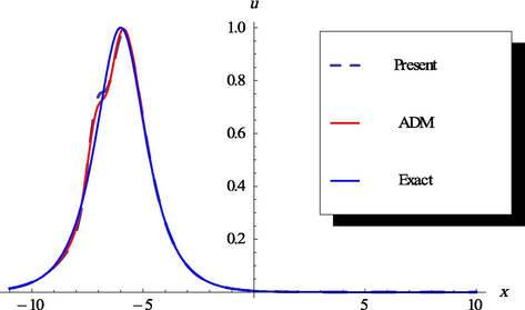
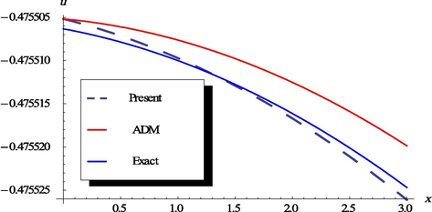
and so on. The behavior of the two solutions given by the presented scheme and that of the ADM for certain values of time is depicted and compared with the exact solutions in Figs. 10 and 11. Besides, the exact solutions of $u\left(x,t\right)$ and $v\left(x,t\right)$ were previously given in (Schiesser, 1994) as $$u\left(x,t\right)=\frac{1}{2}+\mathrm{T}\mathrm{a}\mathrm{n}\mathrm{h}\left(x+at\right),v\left(x,t\right)=1+\mathrm{T}\mathrm{a}\mathrm{n}\mathrm{h}\left(x+at\right),$$ $$a=\frac{1}{4}\left(-4k^2-6\lambda +\frac{6k\lambda }{\mathrm{b}1}+\frac{3{\mathrm{b}1}^2}{k^2}\right)$$

Close

Fig. 10

The plots of the exact, proposed method and the ADM solution, respectively at t = 0.0, 1.0 and 3.0.

Export to PPT

Close

Fig. 11

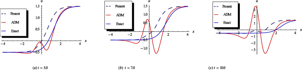
The plots of the exact, proposed method and the ADM solution, respectively at t = 5.0, 7.0 and 10.0.

Export to PPT

5 Conclusion

In conclusion, we have proposed a method based on the recent modification of Adomian decomposition method (ADM) by Zhang and Liang to numerically solve several evolution equations with nonlinearities; particularly the Korteweg de Vries equations. This modification depends on embedding a convergence parameter in the Adomian components. The obtained approximate solutions have been compared to the solutions of the classical AD with the aid of the Mathematica software. The investigated examples show that better accuracy was achieved by the proposed method when compared with those by the ADM for the same number of solution components. The proposed scheme should be considered for extension to other classes of partial differential equations arising in engineering applications.