

Translate this page into:
Mathematical and numerical study of the concentration effect of red cells in blood
-
Received: ,
Accepted: ,
This article was originally published by Elsevier and was migrated to Scientific Scholar after the change of Publisher.
Peer review under responsibility of King Saud University.
Abstract
In this paper, a mathematical and numerical study of the effect of red blood cell concentration on a circular cross-section tube is presented. The considered PDE system use the Bingham model describing blood as a non-Newtonian fluid. This system consists of Navier-Stokes equations describing the behavior of fluid and advection-reaction-diffusion equations that take into account the influence of chemical reactions on transient flow behavior in the arteries. In particular, we present for this problem a local existence result. Finally, numerical tests are presented to treat blood flow in the case of fusiform aneurysms caused by abdominal aortic aneurysm disease.
Keywords
35D30
65N22
76Z05
Bingham model
Advection-diffusion-reaction equation
Abdominal aortic aneurysm
Papanastasiou regularization

1 Introduction
The study of the behavior of fluids according to their viscosity is one of the interesting physical problems. Viscosity is a very important parameter that characterizes the behavior of the fluid since it links the stress of a fluid in motion with the rate of deformation of their constituent elements. For this reason, researchers are increasingly using generalized fluid models to meet the specific needs of modeling, such as the non-Newtonian fluids, which the viscosity cannot be defined as a constant value because of the non-linear relation between the strain rate and the shear stress (Gijsen et al., 1999). If the non-Newtonian character is manifested by the decreasing of the viscosity with increasing shear rate, then it is in the case of rheofluidifiant fluids (or pseudoplastic) (Kim, 2002; Chamekh and Elzaki, 2018).
In this study, we treat the equations modeling the blood behavior in the abdominal aorta in case of an aneurysm involving the non-Newtonian model of Bingham. This modeling is based on the biochemical problem of blood flow in Abdominal Aortic Aneurysms diseases (AAA) (Campa et al., 1987; Goodall et al., 2001; Hallin et al., 2001). It is described by the convection-diffusion-reaction phenomenon, whose blood is considered as an incompressible and rigid viscoplastic fluid with a yield stress of Bingham taking into account the concentration effect of red cells. Then, a result of existence and uniqueness of a maximum principle is proposed for the concentration corresponding to this problem in a three-dimensional delimited domain, also some preliminary and notations found in Messelmi (2014) and Merouani and Messelmi (2015). In the last part, we simulate the blood flow in AAA regularized by Papanastasiou and some numerical results on velocity field and concentration of red cells in AAA are presented.
2 Biological background
Blood is probably the most important biological fluid and its rheology is interesting from both a theoretical and applied point of view. It is a concentrated suspension of several species of particles in the plasma. It contains almost of figurative elements in volume and plasma (Marieb, 1993; Robertson et al., 2008; Brujan, 2010; Toungara, 2011). In the , we find of red blood cells or erythrocytes, and the other are distributed between white blood cells or leucocytes and platelets or thrombocytes (Marieb, 1993; Robertson et al., 2008; Toungara, 2011). Therefore, the red blood cells give a rheological behavior of blood (Robertson et al., 2009; Brujan, 2010). It is well known that blood is an incompressible Newtonian fluid (Gijsen et al., 1999; Paramasivam et al., 2010; Janela et al., 2010).
In general, the natural evolution of AAA differs between humans (Mofidi et al., 2006; DeRubertis et al., 2007). The risk of re-offending is for aneurysms between and in diameter and for aneurysms less than (Khanafar et al., 2006; Paramasivam et al., 2010). There are many constitutive models that are more complex used to study blood flow as the law of power or Cross (Johnstona et al., 2004; Robertson et al., 2008; Messelmi, 2011). More recently, the Bingham model has been used in the modeling of blood flow to describe its behavior through threshold stress and blocking phenomena that describe blood clotting, formation, and lysis of blood clots. We can find in several works on the phenomena of convection-diffusion-reaction which make the study of the coagulation and the formation of blood clots (Merouani and Messelmi, 2015; Hansen et al., 2015; Anand et al., 2003). To do this study, we consider a mathematical model that describes the flow of blood involving the non-Newtonian model of Bingham.
3 Problem description
The purpose of our analysis is to determine the effect of red blood cell concentration on blood behavior. In order to guarantee this, we consider an incompressible flow inside a domain ( ) an open bounded Lipschitzian boundary is the space of the symmetric tensors of order on . The blood temperature is assumed constant. For this problem, viscosity, yield strength, and diffusivity are supposed to depend on the concentration of red blood cells.
Let the space and are equipped by their usual scalar product and Euclidean norm, respectively. For a velocity field , we consider the deformation rate tensor defined by
The equation of fluid motion is given by
The model of Bingham is characterized by
Further, if we assume that the advection convection phenomena of the fluid undergo a chemical reaction under isothermal conditions, then the equation governing the concentration C is given by
The nonlinear advection – diffusion – reaction problem for stationary Bingham fluid is modeled by the partial differential system which consists in finding:
-
the velocity field ,
-
the field of constraints ,
-
the concentration ,
4 Variational formulation
To determine the variational formulation that corresponds to the problem ((1)–(5)). We consider the following space H defined by
where H is a Hilbert space with a scalar product and an induced norm, respectively,
The set H is Banach space. We introduce the following operators
We assume the following hypothesis
5 Existence of solution
The proof of existence is based on the application of Schauder’s fixed point theorem, using in this framework an auxiliary existence result obtained in Kim (1987) and Kim (2002).
To begin, for the operator B and E, we have the following proprieties.
See (Lions, 1969)
(i)The operator B is trilinear, continuous on and for all we have
(14)(ii)The operator E is trilinear, continuous on and
(15)
We have a first result of existence.
For
, it exists a unique solution
of the problem
Let
is the solution of problem (16). Then, it exists a unique solution
of
Let
the following bilinear form
The trilinear operator E is continuous on
. In fact, using the Hölder inequality and Poincaré theorem, we have
Then, we obtain
In addition, by (15), we remark that . Then,
, using in addition that (8), we have the coercivity of . Adding that is lineair continuous by Poincaré formula, we have Using Lax-Milgrame theorem on , then, the problem (23) have a unique solution .
To get auxiliary solution of problem (18), we consider the following operator
Using , then, . Therefore We have Then,
, with
We can write The operator is contracting in the space . So, according to Banach’s fixed point theorem admits a fixed point that we denote which gives .
Then, the fixed-point uniqueness gives which also gives , which implies that the Eq. (18) has a unique solution .
Finding now the estimate (19). We choose as a test function of the Eq. (18). Therefore, we have Using the Hölder inequality, we obtain Using the Poincaré inequality, we obtain Therefore, So, we obtain
6 Numerical treatment
In literature, the Papanastasiou model (Papanastasiou, 1987) of regularization has been widely used in numerical simulations of flows of viscoplastic fluids (Glowinski et al., 2010; Messelmi, 2014; Paramasivam et al., 2010; Soto et al., 2010). The Papanastasiou-Bingham model is as follows:
We will consider now the problem ((1)–(5) with replacing (3) by (25)). The goal is treated this problem numerically simulation. To do this, here and below, we suppose that fluid is stationary, laminar, viscoplastic and incompressible. We suppose that the volume forces are negligible in front of the forces of viscosity, the blood diffusion coefficient
, the yield stress g and the blood viscosity
do not depend on the concentration, except the Reaction function that is nonlinear and generally has an unknown expression. According to the bio-mechanical problem ((1)–(5) with replacing (3) by (25)), the variational formulation is as follows
6.1 Numerical results
This section focuses on the 2D numerical study of the effect of concentration of blood cell in fusiform aneurysms caused by the AAA diseases in two-dimensional model. We use in this study two types of geometries of an Abdominal Aortic Aneurysms, one presents a fusiform aneurysm caused by the AAA diseases without bifurcation and with bifurcation (Fig. 1). It represents a fusiform AAA with a bifurcation at the level of the abdominal aorta, which is split into two iliac arteries. The AAA models have a aorta diameter
, the maximum diameter,
, a length,
. The diameter of each output of the right and left branches of the bifurcation is
. The order of the average velocity of blood is
, since it does not circulate at the same velocity throughout the body. The meshes were built with Freefem++ software. We found that the
component of the velocity along
varies nonlinearly between
and
, while the
component
and
for a high rate of shear that due to a very low viscosity
. In this state, we can conclude that blood behaves like a Newtonian fluid. This shows that the main flow is relatively dominated by the
component. The resolution is done by varying the number of meshes to test the convergence using triangular finite elements. The velocity is computed throughout aneurysmal fusiform at a variable rate of shear which respectively to the deformation of the red blood cell rolls on both models of AAA, shown in Fig. 2.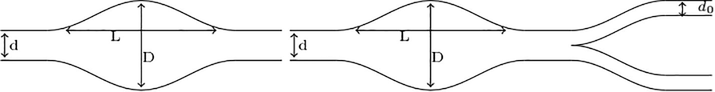
Fusiform aneurysms caused by the AAA diseases without and with bifurcation.
![The velocity profiles u x on x ∈ [ 0 , L ] for the fusiform AAA model without bifurcation, the left figure for a low rate ( μ = 0.00345 Pa s ) and the right figure for a high rate ( μ = 0.056 Pa s ) .](/content/185/2019/31/4/img/10.1016_j.jksus.2018.11.004-fig2.png)
The velocity profiles
on
for the fusiform AAA model without bifurcation, the left figure for a low rate
and the right figure for a high rate
.
The solutions of the velocity for different numbers of meshes, Fig. 2 are obtained in a compatible way, which makes it possible to conclude to the convergence. For both models with or without bifurcation of AAA disease, a remarkable change in velocity component with a relatively high viscosity can be observed, than to the case of a shear rate due to a lower viscosity .
We set the number of meshes at
. The velocity component
for both models and in both cases low and high shear rates are confounded, see Fig. 3, which shows the convergent even if we let us change the regularization values. We noted in the case of AAA without bifurcation, when the shear rate is relatively low the value of
is almost constant in the first half of the aneurysm fusiform
, then this value increases remarkably in the second half. This increase does not appear in the same way when the viscosity is relatively low. On the other hand, for the bifurcated model, there is a remarkably large change in speed for the case of a low shear rate compared with the case of a high rate. We have noticed that the smallest regularization value we can take to get convergent solutions for the AAA model without bifurcation is
and
for the other. This can influence the reasonableness of the result obtained, since it takes the value of regularization to be small to obtain precise solutions. In what follows, we are interested in the study of blood flow in the aneurysmal fusiform with velocity distribution analysis in the aorta. Fig. 4 shows the velocity profiles of an AAA with and without bifurcation for a high and low shear rate. Comparing the results, we find that both models of the AAA have the same velocity profiles for a low viscosity
. That was not the case for a low shear rate.![The velocity profiles u x on the domain x ∈ [ 0 , L ] for the fusiform AAA model, the left figure for a low rate ( μ = 0.056 Pa s ) and the right figure for a high rate ( μ = 0.00345 Pa s ) .](/content/185/2019/31/4/img/10.1016_j.jksus.2018.11.004-fig3.png)
The velocity profiles
on the domain
for the fusiform AAA model, the left figure for a low rate
and the right figure for a high rate
.
![The velocity profiles u x on the domain x ∈ [ 0 , L ] for a low and high rate, the left figure for the fusiform AAA model without bifurcation and the right figure for the fusiform AAA model with bifurcation.](/content/185/2019/31/4/img/10.1016_j.jksus.2018.11.004-fig4.png)
The velocity profiles
on the domain
for a low and high rate, the left figure for the fusiform AAA model without bifurcation and the right figure for the fusiform AAA model with bifurcation.
7 Discussions
When we treat the flow of blood and its viscosity, we talk about the concentration of red blood cells. It varies between 130 and
in a healthy man and between 110 and
in a woman. From the Fig. 5, we notice that the concentrations corresponding to the previous velocities for a high shear rate of two models decrease. On the other hand, for a very high viscosity, the concentration of hemoglobin throughout the hump remains stable at very important values for the two models of AAA with or without a bifurcation. This increase can produce a blockage of blood flow at this hump. On the one hand, for blood pressure Fig. 5, it is almost the same situation for both models of AAA at low viscosity. On the other hand, it is obviously important in the presence of the bifurcated geometry of the aorta. We can conclude that when the velocity is in the stage of acceleration Fig. 4, the pressure will be strongly increasing (5). This phenomenon characterizes blood modeled as Bingham fluid. This is shown in Fig. 5 for pressure in case of a low shear rate of the AAA model with bifurcation. Moreover, this shows the great influence of decay of the viscosity and thus the growth of concentration on pressure and velocity.![The pressure that corresponds to the velocity profiles u x on the domain x ∈ [ 0 , L ] for a low and high rate, the left figure for the fusiform AAA model without bifurcation and the right figure for the fusiform AAA model with bifurcation.](/content/185/2019/31/4/img/10.1016_j.jksus.2018.11.004-fig5.png)
The pressure that corresponds to the velocity profiles
on the domain
for a low and high rate, the left figure for the fusiform AAA model without bifurcation and the right figure for the fusiform AAA model with bifurcation.
References
- Model incorporating some of the mechanical and biochemical factors underlying clot formation and dissolution in flowing blood. J. Theor. Med.. 2003;5:183-218.
- [Google Scholar]
- Cavitation in Non-Newtonian Fluids: With Biomedical and Bioengineering Applications. Springer Science & Business Media; 2010. p. :269.
- Explicit solution for some generalized fluids in laminar flow with slip boundary conditions. J. Math. Comput. Sci.. 2018;18:72-281.
- [Google Scholar]
- Abdominal aortic aneurysm in women: prevalence, risk factors, and implications for screening. J. Vasc. Surg.. 2007;46(4):630-635.
- [Google Scholar]
- The influence of the non-Newtonian properies of blood on the flow in large arteries: unsteady flow in a 90 curved tube. J. Biomech.. 1999;32:705-713.
- [Google Scholar]
- Numerical Methods for Non-Newtonian Fluids. 16: Special Volume (Handbook of Numerical Analysis) 2010
- Ubiquitous elevation of matrix metalloproteinase-2 expression in the vasculature of patients with abdominal aneurysms. Circulation. 2001;104(3):304-309.
- [Google Scholar]
- Literature review of surgical management of abdominal aortic aneurysm. Eur. J. Vasc. Endovasc. Surg.. 2001;22(3):197-204.
- [Google Scholar]
- Mechanical platelet activation potential in abdominal aortic aneurysms. J. Biomech. Eng. 2015:137.
- [Google Scholar]
- A 3D non-Newtonian fluid structure interaction model for blood flow in arteries. J. Comput. Appl. Math.. 2010;234:2783-2791.
- [Google Scholar]
- Non-Newtonian blood flow in human right coronary arteries: steady state simulations. J. Biomech.. 2004;37:709-720.
- [Google Scholar]
- Modeling pulsatile flow in aortic aneurysms: effect of non-Newtonian properties of blood. Biorheology. 2006;43:661-679.
- [Google Scholar]
- On the initial-boundary value problem for a Bingham fluid in a three-dimensional domain. Trans. Am. Math. Soc.. 1987;304(2):751-770.
- [Google Scholar]
- A study of non-newtonian viscosity and yield stress of blood in a scanning capillary-tube rheometer. Drexel University; 2002. (A Thesis)
- Quelques méthodes de résolution des problèmes Aux limites non linéaires. Paris: Dunod; 1969.
- Anatomie et physiologie humaines. De Boeck Université; 1993.
- Existence of weak solutions for the quasi-state flow of blood and mathematical coagulation modeling. Nonlinear Funct. Anal. Appl.. 2015;20(3):393-418.
- [Google Scholar]
- Diffusion-reaction problem for the Bingham fluid with Lipschitz Source. Int. J. Adv. Appl. Math. Mech.. 2014;1(3):37-55.
- [Google Scholar]
- The existence of weak solutions for the 3D-steady-state flow of blood in arteries. Fasc. Matematica Tom. 2011;XVIII:221-240.
- [Google Scholar]
- Influence of sex on expansion rate of abdominal aortic aneurysms. Br. J. Surg.. 2006;94:310-314.
- [Google Scholar]
- Finite element modeling for solving the pulsatile flow in a fusiform abdominal aortic aneurysm. Biomed. Int.. 2010;1(2):50-61.
- [Google Scholar]
- Elastin degradation in abdominal aortic aneurysms. Atherosclerosis. 1987;65(1–2):13-21.
- [Google Scholar]
- Robertson, A.M., Rannacher, R., Galdi, G.P., Turek, S., 2008. Hemodynamical flows. Modeling, analysis and simulation. In: Oberwolfach Seminars. 37, Birkhauser. p. 501.
- Rheological models for blood. In: Quarteroni A., Formaggia L., Veneziani A., eds. Cardiovascular Mathematics. Modeling and Simulation of the Cardiovascular System. Vol vol. 1. A. Springer-Verlag; 2009.
- [Google Scholar]
- A numerical investiion of inertia flows of Bingham-Papanastasiou fluids by an extra stress-pressure-velocity galerkin least-squares method. J. Braz. Sgatoc. Mech. Sci. & Eng. 2010;32 no.spe Rio de Janeiro
- [Google Scholar]
- Contribution à la prdiction de la rupture des Anévrismes de l’Aorte Abdominale (AAA). Life Sciences. Universié de Grenoble; 2011. Thèse de doctorat


