

Translate this page into:
Non-polynomial quadratic spline method for solving fourth order singularly perturbed boundary value problems
-
Received: ,
Accepted: ,
This article was originally published by Elsevier and was migrated to Scientific Scholar after the change of Publisher.
Peer review under responsibility of King Saud University.
Abstract
In this paper, a non-polynomial quadratic spline method is described for solving fourth-order boundary value problems whose highest-order derivative is multiplied by a small perturbation parameter. This method is applied directly to the solution of the problem without reducing the order of the problem. Convergence analysis of the fourth order method is discussed. To illustrate the efficiency of the method, a boundary value problem is considered with different type of boundary conditions and obtained numerical results are compared with the existing methods.
Keywords
Fourth order singularly perturbed boundary value problems
Non-polynomial quadratic spline
Convergence analysis

1 Introduction
Fourth order singularly perturbed boundary value problems occur frequently in many areas of applied sciences such as solid mechanics, Newtonian fluid mechanics, chemical reactor theory, aerodynamics, hydrodynamics, optimal control, convection diffusion processes, quantum mechanics, etc. These problems have various important applications in fluid dynamics. Ghasemi et al. (2014) gave the analysis of electrohydrodynamic flow in a circular cylindrical conduit using least square method and Hatami and Domairry (2014) investigated the transient vertically motion of a soluble particle in a Newtonian fluid media. Hatami and Ganji (2014) studied the motion of a spherical particle in a fluid forced vortex by DQM and DTM. Hatami et al. (2016) gave the optimization of a circular-wavy cavity filled by nanofluid under the natural convection heat transfer condition. Nadeem and Haq (2014) studied the effect of thermal radiation for megnetohydrodynamic boundary layer flow of a nanofluid past a stretching sheet with convective boundary conditions. Sheikholeslami and Ganji investigated the nanofluid flow and heat transfer between parallel plates considering Brownian motion using DTM in Sheikholeslami and Ganji (2015). Sheikholeslami et al. (2013) gave investigation of squeezing unsteady nanofluid flow using ADM. Sheikholeslami et al. (2012) discussed analytical investigation of Jeffery-Hamel flow with high magnetic field and nanoparticle by Adomian Decomposition Method. Sheikholeslami et al. (2012) investigated the laminar viscous flow in a semi-porous channel in the presence of uniform magnetic field using Optimal Homotopy Asymptotic Method. Zhou et al. (2016) designed the microchannel heat sink with wavy channel and its time-efficient optimization with combined RSM and FVM methods.
Singularly perturbed problems are classified on the fact that how the order of the differential equation is affected if , here is a small positive parameter multiplying the highest order derivative of the differential equation. The solution of singularly perturbed boundary value problem has a multiscale character; that is, there are thin transition layers where the solution varies rapidly, while away from the layers the solution varies very slowly.
In this paper, we develop a computational method to solve fourth order singularly perturbed boundary value problems of the form:
OR
In literature, we found many numerical methods which were developed for solving second order singularly perturbed BVPs. These methods are exponentially fitted finite difference scheme (Kadalbajoo and Kumar, 2009), non-polynomial spline method (Tirmizi, 2008), cubic spline method (Kumar et al., 2007) and quintic spline method (Rashidinia et al., 2010) etc. There are few methods available for solving higher order singularly perturbed BVPs such as asymptotic finite element method (Babu and Ramanujam, 2007), reproducing kernel method (Akram and Rehman, 2012). Shanthi and Ramanujam (Shanthi and Ramanujam, 2002) solved singularly perturbed fourth-order ordinary differential equations of convection–diffusion type using asymptotic numerical methods. The authors in Akram and Amin (2012, 2013) used quintic spline and septic spline respectively for solving fourth order singularly perturbed BVPs.
However, most of these methods were used to solve fourth-order singularly perturbed boundary value problem by using a higher degree spline. Here, we use a non-polynomial quadratic spline method for solving the problem (1). In this paper, we discuss two types of boundary value problems with boundary conditions (2) and (3). Firstly a numerical system is obtained by using non-polynomial quadratic spline. Then finite difference formula of is used for making the system consistent with the given boundary value problem. Finally the obtained scheme is used to solve fourth order singularly perturbed boundary value problems. After implementation of the problem over the method we get a system of pentadiagonal matrix which is solved by using LU decomposition method. The paper describing a non-polynomial quadratic spline method is organized into five sections. Section 2 gives a brief derivation of the method, along with boundary conditions. In Section 3 truncation error has been obtained for fourth order method. Application of the method for solving fourth order singularly perturbed BVPs is discussed in Section 4. Convergence analysis of the method is discussed in Section 5. In Section 6, numerical examples and their comparison with the existing methods are presented which demonstrate the efficiency of our method. Conclusion and the figures are presented in Section 7 also proves the accuracy.
2 Derivation of the scheme
Let , we first divide the interval [a,b] into equal parts by introducing
Let
To determine the coefficients
, we define the following interpolatory conditions as
By using above conditions we calculated the coefficients as where,
Using the continuity of first derivative,
the following consistency relation is derived
Our method reduces to Al-Said (2008) based on quadratic spline when
For making the system consistent with the given boundary conditions, we use finite difference formula of
Using (6) and (8), we obtained the following relation
Eq. (9) form a system of linear equations in n unknowns . Thus, we need two more equations, one at each end of the range of integration.
For case (i), the equations are obtained as
For case (ii), the equations are obtained as
3 Truncation error
Expanding (9) by using Taylor series, we obtained the following truncation error
For different values of parameters, we get the method of second order as well as fourth order. Here we discuss only fourth order method. The local truncation error for (10) and (11) is and the local truncation error for (12) and (13) is
For the truncation error is
4 Application to the fourth order singularly perturbed boundary value problems
We consider a fourth order singularly perturbed boundary value problem of the form subject to the boundary conditions
OR where are sufficiently continuously differentiable functions in the interval and are real constants.
After applying the scheme (9) to the problem (1) with boundary conditions (2) and (3), we get the following relation
Eqs. (10) and (11) takes the form where,
Eqs. (12) and (13) takes the form where,
5 Convergence analysis
The developed method leads to the following matrix form
and the right hand side vector is .
For Case (i), we have
For Case (ii),we have
Also we have,
A pentadiagonal matrix , where for , is irreducible iff
Now we have to calculate sum of each row of matrix P:
For case (i),
For case (ii),
Let is the minimum of . For sufficiently small h we can say that:
For case (i),
For case (ii),
Further,we get for case (i)
For sufficiently small h, we can easily show that the matrix P is irreducible and monotone. Therefore,
exist and
. Hence,
Therefore, and error is given by:
For case (i),
Similarly for Case (ii), the error is given by
By using (14), we have truncation error , then we get
Hence, the scheme is fourth order convergent.
The method given by Eq. (9) for solving the given singularly perturbed boundary value problem for sufficiently small h has a fourth order convergence.
6 Numerical illustrations
In the present paper, we consider two linear fourth order singularly perturbed boundary value problems whose exact solutions are known. The maximum absolute errors for h = 1/16, 1/32, 1/64 and 1/128 are tabulated in Tables 1 and 2 and comparison are also shown in graphs 1–2. The obtained results are compared with the results of quintic spline method (Akram and Amin, 2012) and septic spline method (Akram and Naheed, 2013).
For
, consider the following differential equation:
For
, consider the following differential equation:
Maximum absolute errors for Example 2 are given in Table 2. For the sake of comparison we are also reported results of Akram and Amin (2012) and Akram and Naheed (2013) in the Table 2.
| Our method | |||||
| Akram and Amin (2012) | |||||
| Our method | |||||
| Akram and Amin (2012) | |||||
| Our method | |||||
| Akram and Amin (2012) | |||||
| Our method | |||||
| Akram and Amin (2012) | 6.682 × 10(-9) | ||||
| Akram and Naheed (2013) | |||||
| Our method | |||||
| Akram and Amin (2012) | |||||
| Akram and Naheed (2013) | |||||
| Our method | |||||
| Akram and Amin (2012) | |||||
| Akram and Naheed (2013) | |||||
| Our method | |||||
| Akram and Amin (2012) | |||||
| Akram and Naheed (2013) | |||||
7 Conclusion
Non-polynomial quadratic spline method is developed for the approximate solution of fourth order singularly perturbed boundary value problems with two types of boundary conditions. Convergence analysis of the method proved that our scheme (9) is fourth order convergent. A lower degree non-polynomial quadratic spline is used in this paper. However, in previous papers higher degree quintic and septic splines were used. This method is also applicable to solve linear boundary value problems as
. Maximum absolute errors in Tables 1 and 2 shows that our method is better than existing methods. Graphs between exact and approximate solutions for the Examples 1 and 2 are shown in Fig. 1 and 2 respectively which also shows the superiority of our method.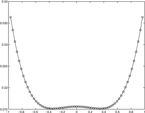
Graph of the exact solution versus the approximate solution for N = 64 for Example 1.
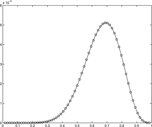
Graph of the exact solution versus the approximate solution for N = 64 for Example 2.
Acknowledgement
The second author is thankful to UGC for providing MANJRF. The authors are also thankful to the referees for useful suggestions which improve the quality of the paper.
References
- Solution of a fourth order singularly perturbed boundary value problem using quintic spline. Int. Math. Forum. 2012;7:2179-2190.
- [Google Scholar]
- Solution of fourth order singularly perturbed boundary value problem using septic spline. Middle-East J. Sci. Res.. 2013;15:302-311.
- [Google Scholar]
- Reproducing kernel method for fourth order singularly perturbed boundary value problem. World Appl. Sci. J.. 2012;16:1799-1802.
- [Google Scholar]
- Quadratic spline method for solving fourth order obstacle problems. Appl. Math. Sci.. 2008;2:1137-1144.
- [Google Scholar]
- An asymptotic finite element method for singularly perturbed third and fourth order ordinary differential equations with discontinuous source term. Appl. Math. Comput.. 2007;191:372-380.
- [Google Scholar]
- Electrohydrodynamic flow analysis in a circular cylindrical conduit using least square method. J. Electrostat.. 2014;72:47-52.
- [Google Scholar]
- Transient vertically motion of a soluble particle in a Newtonian fluid media. Powder Technol.. 2014;253:481-485.
- [Google Scholar]
- Motion of a spherical particle in a fluid forced vortex by DQM and DTM. Particuology. 2014;16:206-212.
- [Google Scholar]
- Optimization of a circular-wavy cavity filled by nanofluid under the natural convection heat transfer condition. Int. J. Heat Mass Transfer. 2016;98:758-767.
- [Google Scholar]
- Initial value technique for singularly perturbed two point boundary value problems using an exponentially fitted finite difference scheme. Comput. Math. Appl.. 2009;57:1147-1156.
- [Google Scholar]
- An initial-value technique for singularly perturbed boundary value problems via cubic spline. Int. J. Comput. Methods Eng. Sci. Mech.. 2007;8:419-427.
- [Google Scholar]
- Ul, Effect of thermal radiation for megnetohydrodynamic boundary layer flow of a nanofluid past a stretching sheet with convective boundary conditions. J. Comput. Theor.Nanosci.. 2014;11:32-40.
- [Google Scholar]
- Quintic spline methods for the solution of singularly perturbed boundary-value problems. Int. J. Comput. Methods Eng. Sci. Mech.. 2010;11:247-257.
- [Google Scholar]
- Asymptotic numerical method for singularly perturbed fourth-order ordinary differential equations of Convection-diffusion type. Appl. Math. Comput.. 2002;133:559-579.
- [Google Scholar]
- Nanofluid flow and heat transfer between parallel plates considering Brownian motion using DTM. Comput. Methods Appl. Mech. Eng.. 2015;283:651-663.
- [Google Scholar]
- Investigation of squeezing unsteady nanofluid flow using ADM. Powder Technol.. 2013;239:259-265.
- [Google Scholar]
- Analytical investigation of Jeffery-Hamel flow with high magnetic field and nanoparticle by Adomian decomposition method. Appl. Math. Mech.. 2012;33:25-36.
- [Google Scholar]
- Investigation of the laminar viscous flow in a semi-porous channel in the presence of uniform magnetic field using Optimal Homotopy Asymptotic Method. Sains Malaysiana. 2012;41:1281-1285.
- [Google Scholar]
- Non-polynomial spline solution of singularly perturbed boundary-value problems. Appl. Math. Comput.. 2008;196:6-16.
- [Google Scholar]
- Matrix Iterative Analysis. Englewood Cliffs, NJ: Prentice-Hall; 1962.
- Design of microchannel heat sink with wavy channel and its time-efficient optimization with combined RSM and FVM methods. Int. J. Heat Mass Transfer. 2016;103:715-724.
- [Google Scholar]


