Translate this page into:
An ensemble of classifiers based on different texture descriptors for texture classification
*Corresponding author. Tel.: +39 3493511673 loris.nanni@unibo.it (Loris Nanni)
-
Received: ,
Accepted: ,
This article was originally published by Elsevier and was migrated to Scientific Scholar after the change of Publisher.
Abstract
Here we propose a system that incorporates two different state-of-the-art classifiers (support vector machine and gaussian process classifier) and two different descriptors (multi local quinary patterns and multi local phase quantization with ternary coding) for texture classification.
Both the tested descriptors are an ensemble of stand-alone descriptors obtained using different parameters setting (the same set is used in each dataset). For each stand-alone descriptor we train a different classifier, the set of scores of each classifier is normalized to mean equal to zero and standard deviation equal to one, then all the score sets are combined by the sum rule.
Our experimental section shows that we succeed in building a high performance ensemble that works well on different datasets without any ad hoc parameters tuning. The fusion among the different systems permits to outperform SVM where the parameters and kernels are tuned separately in each dataset, while in the proposed ensemble the linear SVM, with the same parameter cost in all the datasets, is used.
Keywords
Machine learning
Non-binary coding
Support vector machine
Ensemble of classifiers
Texture descriptors
1 Introduction
The importance of texture analysis as a branch of computer vision has been cleared from decades (Haralick et al., 1973)and its range of applications is dramatically wide, from medical image processing (Vécsei et al., 2011) to face recognition (Tan and Triggs, 2010).
The success of texture analysis is easily understandable since almost every image contains texture and the continuous development in image acquisition technology made high-resolution pictures more available. Texture analysis is important in many machine learning problems, including medical image analysis, surface inspection, and a host of image detection and classification problems. As a result of extensive research on texture analysis over the last 30 years, the literature is rich with techniques for describing image textures (Xie and Mirmehdi, 2008).
Of note, even if various different qualitative definitions of texture were published and intuitively it is easy thinking about what a texture is, there is no univocal quantitative definition. Different attempts are reported in the literature (Tamura and Mori, 1978; Sklansky, 1978; Haralick, 1979; Hawkins, 1969) and reviewed in Tuceryan (1998): the common basic elements emerging from these sources are (i) the presence of repetitive primitives (patterns) having the same size everywhere in the textured region and (ii) the spatial non-random organization of these primitives in a region larger in comparison with the primitive size itself.
In spite of the lack of a formal quantitative texture definition, a variety of quantitative texture descriptors was developed during the last forty years: in Fernández et al. (2012) a classification of the most relevant texture descriptors based on histograms of equivalent patterns is provided discriminating between global and local methods, i.e. texture descriptors taking into account or not, respectively, parameters computed from the whole image such as a global threshold used for binarization.
Among the local texture descriptors we report the most used approaches (i) methods based on the gray level co-occurrence matrix (GLCM), which measures the joint probability of the gray levels at two pixels at a fixed relative position, such as Haralick features (Haralick et al., 1973), where a set of features is computed on GLCMs built according to different orientations and (ii) neighborhood based methods, computed directly on the image using a shifting neighborhood (square, rectangular, circular, etc.). Research on the neighborhood based texture descriptors was extremely prolific from the nineties and a wide spectrum of different methods was proposed such as the Rank Transformations (Zabih and Woodfil, 1994), which considers the neighborhood pixels with lower intensity than the central neighborhood pixel, or the Texture Spectrum (He and Wang, 1990) and its simplified version (Xu et al., 2003), where a basic ternary coding is used according to the fact that the intensity values of the neighboring pixels are lower, equal or higher than the central pixel value. Local Binary Patterns (LBP) Ojala et al., 2002 is an extremely versatile descriptor, as we detail in the method section, and it was exploited in diverse applications and evolved into different new operators such as Local Ternary Patterns (Tan and Triggs, 2010), Local Quinary Patterns (LQP, details in Section 2) (Nanni et al., 2010), Centralized Binary Patterns (Fu and Wei, 2008), Binary Gradient Contours (BGC) Hayman et al., 2004, and Completed Local Binary Patterns (CLBP) Guo et al., 2010. In the CLBP operator, two global sub-operators are used considering two global thresholds based on the gray intensity of the whole image (CLBP_C) and the average difference between peripheral pixel and the central pixel gray levels (CLBP_M), as well as the plain LBP (the third local sub-operator). We include among the local texture descriptors the powerful Local Phase Quantization (LPQ) Rahtu et al., 2012, which is not computed directly on the gray levels of the neighborhood included pixels, but on the phase information extracted from the Fourier transform computed on the neighborhood itself.
Global methods such as the binary Texture Co-occurrence Spectrum (Patel and Stonham, 1991) and Coordinated Cluster Representation (Kurmyshev and Cervantes, 1996) take into account a global threshold (which in the implementation provided in Fernández et al. (2012) is computed as the gray level dividing the image intensity histogram into two parts of equal entropy).
Moreover several works (e.g. Paci et al., 2012) show that a single texture descriptor cannot bring enough information for obtaining good results in difficult datasets. For solving this problem several authors (as in this work) use an ensemble of classifiers combined in some way (e.g. sum rule) Kuncheva, 2004. In the computer vision field the easier way for building an ensemble is to train different classifiers using different texture descriptors. In the present work, starting from our previous results, we propose to combine two different high performance texture descriptors, namely multi-threshold local quinary patterns (MLQP) and multi-threshold local phase quantization with ternary coding (MLPQ3), with two high performance classifiers, i.e. support vector machine (SVM) and gaussian process classifier (GP). In this way we build an ensemble of four approaches (2 texture descriptors × 2 classifiers) combined by the sum rule (Bianconi et al., 2007). The aim of this work is to apply this approach to the wide suite of datasets used by Fernández et al. (2012) in order to assess its effectiveness on different texture datasets.
The paper is organized as follows: in Section 2 the texture descriptors used in our system are briefly reviewed, in Section 3 the classifiers used in our system are explained, in Section 4 details on the tested datasets are provided, in Section 5 experimental results are presented and discussed and finally in Section 6 the conclusions are drawn.
2 Descriptors
2.1 Local quinary patterns (LQP)
The LQP operator represents an improvement of the classical LBP operator (Ojala et al., 2002). The main weakness of the LBP operator is that the binary
function thresholds exactly at the intensity value of the central pixel qc, which makes this operator sensitive to noise especially in near-uniform regions. To overcome this weakness, the quinary coding proposed in Paci et al. (2012) can be used. The quinary coding is achieved introducing two thresholds τ1 and τ2 in the canonical LBP s(x) function which becomes:
To reduce the size of the histogram summarizing the extracted patterns, the original LQP code is thus split into 4 different sets of binary patterns, according to the following binary function bc(x), c ∈ {−2,−1, 1,2}:
Each set of binary patterns is mapped according to the “uniform rotation invariant” (riu2) mapping Ojala et al., 2002 using two neighborhoods: (i) the 8 pixel neighborhood resulting in 10 features and (ii) the 16 pixel neighborhood resulting in 18 features. So the histogram obtained by combining the two neighborhoods is composed by 28 elements.
Finally, these 4 histograms are concatenated to form the feature vector containing 112 bins: 28 (features of each histogram) × 4 (number of histograms).
2.2 Local phase quantization (LPQ) and LPQ with ternary coding (LPQ3)
LPQ is based on the blur invariance of the Fourier Transform Phase (Rahtu et al., 2012), locally computed from the 2D Short Term Fourier Transform (STFT) for each pixel position of the image over a square neighborhood.
Considering the 2D Fourier transforms F of the original picture f, H of the point spread function (PSF) h and G of the blurred image g, they are bounded by the following relation
Thus magnitude and phase aspects can be separated thus resulting in
and
If the blur PSF h is centrally symmetric, its Fourier transform H is always real-valued, and its phase is a two-valued function given by
meaning that F and G have the same phase at those frequencies which make H positive.The LPQ method is based on the above properties of blur invariance. It uses the local phase information extracted using STFT computed over a square neighborhood at each pixel position x of the image f(x). The binary code assignment at each x depends on the phase information only and the phase is computed by observing the component of the Fx vector where and the u vectors frequency vectors are u1 = [a,0]T, u2 = [0,a]T, u3 = [a, a]T, and u4 = [a,−a]T where a is small enough to satisfy H(u) ⩾ 0.We defined Gx = VTFxwhere V is an orthonormal matrix derived from the singular value decomposition of the covariance matrix of the transform coefficient vector Fx. The resulting vectors are quantized: where gj represents the j-th component of Gx. These quantized coefficients are represented as integers between 0 and 255 using the binary coding
These integer values are then organized in the feature vector useful for classification tasks. In this paper we have used a rectangular neighborhood of size 3 and 5 concatenating the two histograms before training a given classifier.
As for LBP a non-binary coding is proposed for the LPQ operator (Paci et al., 2012): in this case the LPQ with ternary coding (LPQ3) uses the following quantizer: where τj is set to half of the standard deviation of the j-th component of Gx, and ρ is the given weight. The quantized coefficients are then represented as integers in the interval 0–255 using the following binary codings
and
b+ and b− values are then summarized in two distinct 256 bins histograms and the two histograms are then concatenated thus providing a 512 valued feature vector (for both the neighborhood of size 3 and 5, i.e. the final feature vector is 1024 bins), useful for classification tasks.
2.3 The multi-threshold approach
The use of ternary and quinary codings requires respectively one (τ) or two (τ1 and τ2) thresholds to be set. The threshold selection is a critical task in order to reduce the sensitivity to noise of these new operators: thresholds were usually set manually in order to get the best performance in specific problems, but some automatic adaptive procedures were also proposed in Vécsei et al. (2011) exploiting local statistics as mean value and standard deviation inside each neighborhood. Another approach lies in choosing a set of different thresholds for the ternary coding (or a set of different couples of thresholds for the quinary coding), in order to (i) extract a different feature set according to each threshold (or couple of thresholds), (ii) use each feature set to train a different classifier and (iii) fuse all these results according to a fusion rule (sum, mean, vote, etc.).
In details, in this work we considered:
25 threshold couples (τ1 = {1,3,5,7,9} and τ2 = {τ1 + 2, …, 11}) for LQP i.e. 25 feature sets;
5 thresholds (τ ∈ {0.2, 0.4, 0.6, 0.8, 1}) for LPQ, i.e. 5 feature sets.
This led to new texture descriptors such as the Multi-threshold Local Quinary Patterns (MLQP) and the Multi-threshold Local Phase Quantization with ternary coding (MLPQ3) Paci et al., 2012.
Since we gathered 30 feature sets we trained 30 different SVMs using one feature set each. For the testing part, after computing the same 30 feature sets from the testing images, each SVM classifies the testing feature set corresponding to the same feature set it was trained with. Then the 30 partial classification results are fused together according to the sum rule (Bianconi et al., 2007). Let us define dt,j(x) the similarity of the pattern x to the class j obtained using the classifier t. The values of dt,j(x) are: real values that represent the distances from the margin when SVM is the classifier; real values varying in the range 0;1 when GPC is the classifier (see Section 3). Before the fusion the set of similarities of each classifier is normalized to mean 0 and standard deviation 1 (Kuncheva, 2004). The sum rule among a pool of T classifiers is the sum among the T set of scores i.e. Sum rule: . Each membership to a class is a sum of real values, so it is almost impossible that a given pattern has the same membership to two (or more) classes1. Each pattern x is assigned to the class with higher membership, i.e. the class of x is argmaxj μj(x).
3 Classifiers
3.1 Support vector machines
Support Vector Machines (SVMs) were first introduced in Vapnik (1995) and are maximum margin classifiers. They are two-class classifiers that find a decision surface by projecting the training samples in the multidimensional feature space and by maximizing the distance of the closest points in the training set to the decision boundary. The goal is to build the hyperplane that maximizes the minimum distance between two classes. Under the hypothesis of linearly separable data
the hypothesis space is summarized in H: fw, b = sgn(w⋅x + b).
In order to maximize the distance
between the training samples and the hyperplane, the function
should be minimized under the constraints
The final form of the decision hyperplane is: where αi and b are the solutions of a quadratic programming problem.
Unknown test data xt can be classified by simply computing:
It can be seen by examining the above equation that the hyperplane is determined by all the training data, xi, that have the corresponding attributes of αi > 0.
In order to get the minimal number of errors during the classification task the constraints can be relaxed, by using the tolerance parameters ξi and the penalty parameter C, in the form
thus changing the function Φ to be minimized as follows:
The final form of the classifier does not change while now 0 ⩽ αi ⩽ C. For more information about SVM, the reader is referred to (Cristianini and Shawe-Taylor, 2000).
We have tested radial basis function and linear kernel, the parameters setting is performed in each dataset. To select the parameters an internal 10-fold cross validation is performed using the training data (so the test set is blind) i.e. each training set is randomly partitioned into 10 equal size subsamples, a single set is retained for testing the model, and the remaining 9 sets are used as a new training set. The cross-validation process is then repeated 10 times (the folds), and the results from the 10 folds are averaged. Using this protocol we select the best parameters for SVM (using a grid search approach as suggested in LibSVM (xxxx)), then these parameters (selected without using the test data) are used to classify test patterns.
3.2 Gaussian process classifiers
A Gaussian process is a generalization of the Gaussian probability distribution. A Gaussian process classifier (GPC) is a discriminative approach where the class membership probability is the Bernoulli distribution (Rasmussen and Williams, 2006). GPC has a proven track record classifying many different tasks.
GPC is based on methods of approximate inference for classification, since the exact inference in Gaussian process models with likelihood functions tailored to classification is intractable. In the rest of this section we use the same symbols and notation from Rasmussen and Williams (2006).
In the basic case of a binary GPC classifier, the main idea consists in introducing a Gaussian Process over the latent function f(x), which is used as the argument of an activation function to get a final output varying in the range 0;1. A commonly used activation function is the logistic function
thus getting a prior on
The inference problem is made of two steps:
-
computing the distribution of f(x) corresponding to a test case where represents the posterior over the latent variables.
-
this distribution over the latent variables is used to produce the prediction for the test case
Due to the non gaussian nature of the posterior p(f|X, y), the first integral is not analitically tractable and approximations have to be used.
The Laplace approximation allows the replacement of p(f|X, y) with its Gaussian approximation around the maximum of the posterior where Following an iterative process to define and A and computing the mean and variance for f∗, the prediction can be written as where q() is gaussian.
Due to execution time we have used default parameters in all the tested datasets2. For more mathematical details of this classification method, the reader would be best served to refer to chapter 3 in Rasmussen and Williams (2006), electronically available at <http://www.gaussianprocess.org/gpml/>. In the experiments we used the code available at <http://www.gaussianprocess.org/gpml/code/matlab/doc/>.
4 Datasets
Eight datasets were considered in this paper. We chose the same datasets used in Fernández et al. (2012), except the Jerry Wu, VisTex and KTH-TIPS2b datasets: in the former 10 images were missed, the second due to execution time, the latter has some texture classes not included into the training set. The following descriptions refer to the dataset versions used by Fernández et al. (2012) and not to the original versions. The main characteristics of each dataset are described in Table 1 (Fernández et al., 2012) and some significant pictures from the datasets are reported in Figs. 1–7.
Dataset
Short name
Classes
Samples/Class
Total samples
Sample resolution
BonnBTF
BO
10
16
160
200 × 200
64 × 64
Brodatz
BR
13
16
208
256 × 256
KTH-TIPS
KT
10
4
40
100 × 100
MondialMarmi
MM
12
64
768
136 × 136
OUTEX_TC_00000
O0
24
20
480
128 × 128
OUTEX_TC_00001
O1
24
88
2112
64 × 64
OUTEX_TC_00013
O3
68
20
1360
128 × 128
UIUCTex
UI
25
40
100
640 × 480
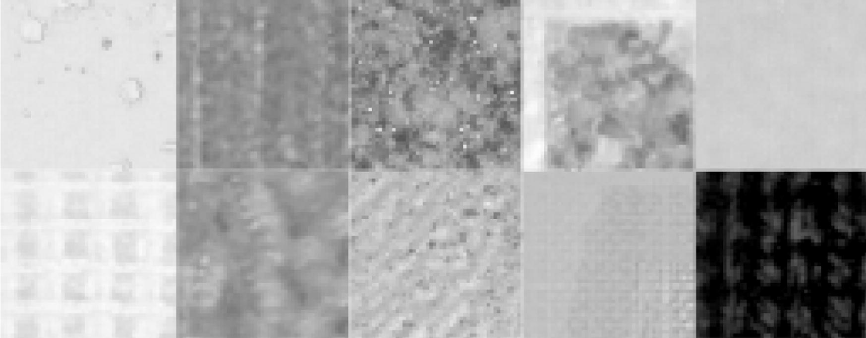
Bonn BTF dataset, 10 classes, (Fernández et al., 2012; Hauth et al., 2002).
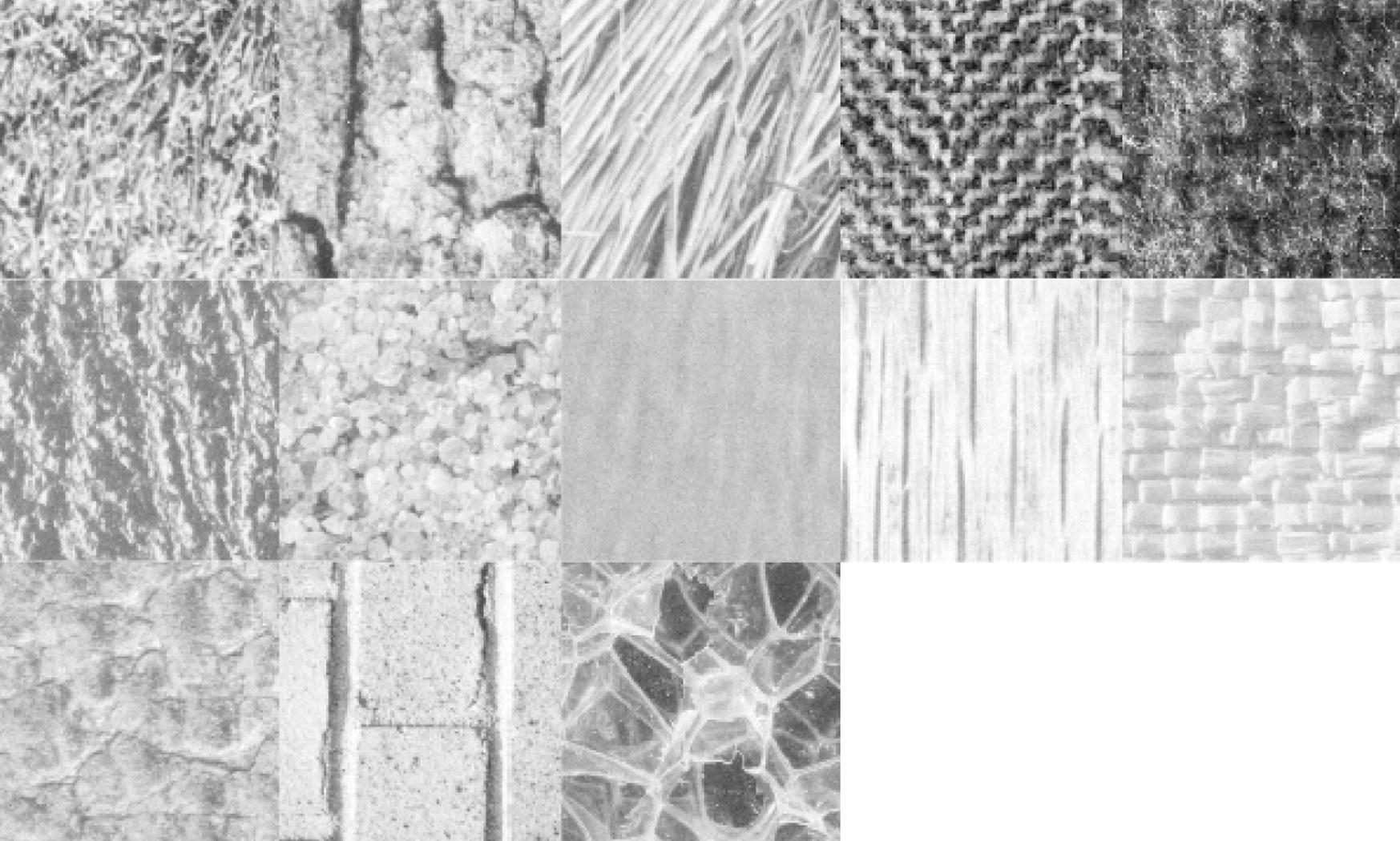
Brodatz dataset, 13 classes, (Fernández et al., 2012; USC-SIPI, xxxx).
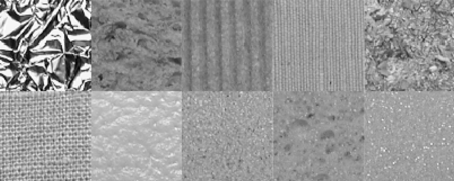
KTH-TIPS dataset, 10 classes, (Fernández et al., 2012; Hayman et al., 2004).
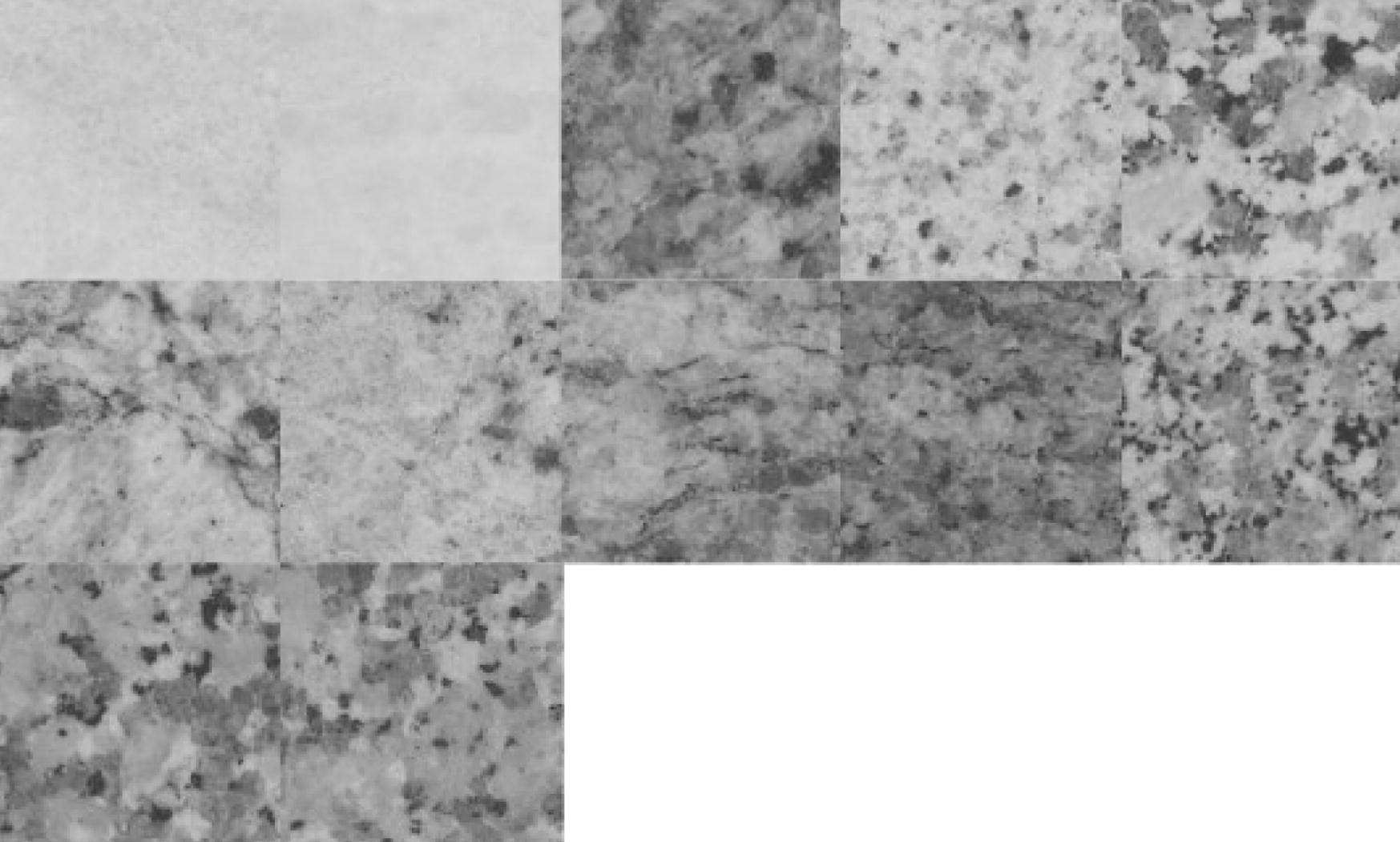
MondialMarmi dataset, 12 classes, (Fernández et al., 2012, 2011b).
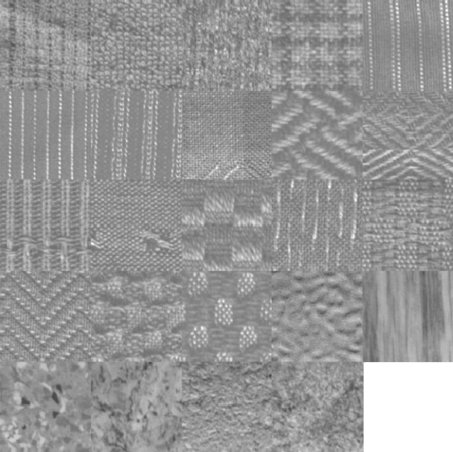
OUTEX TC 00000 dataset, 24 classes, (Fernández et al., 2012; Ojala et al., 2002).
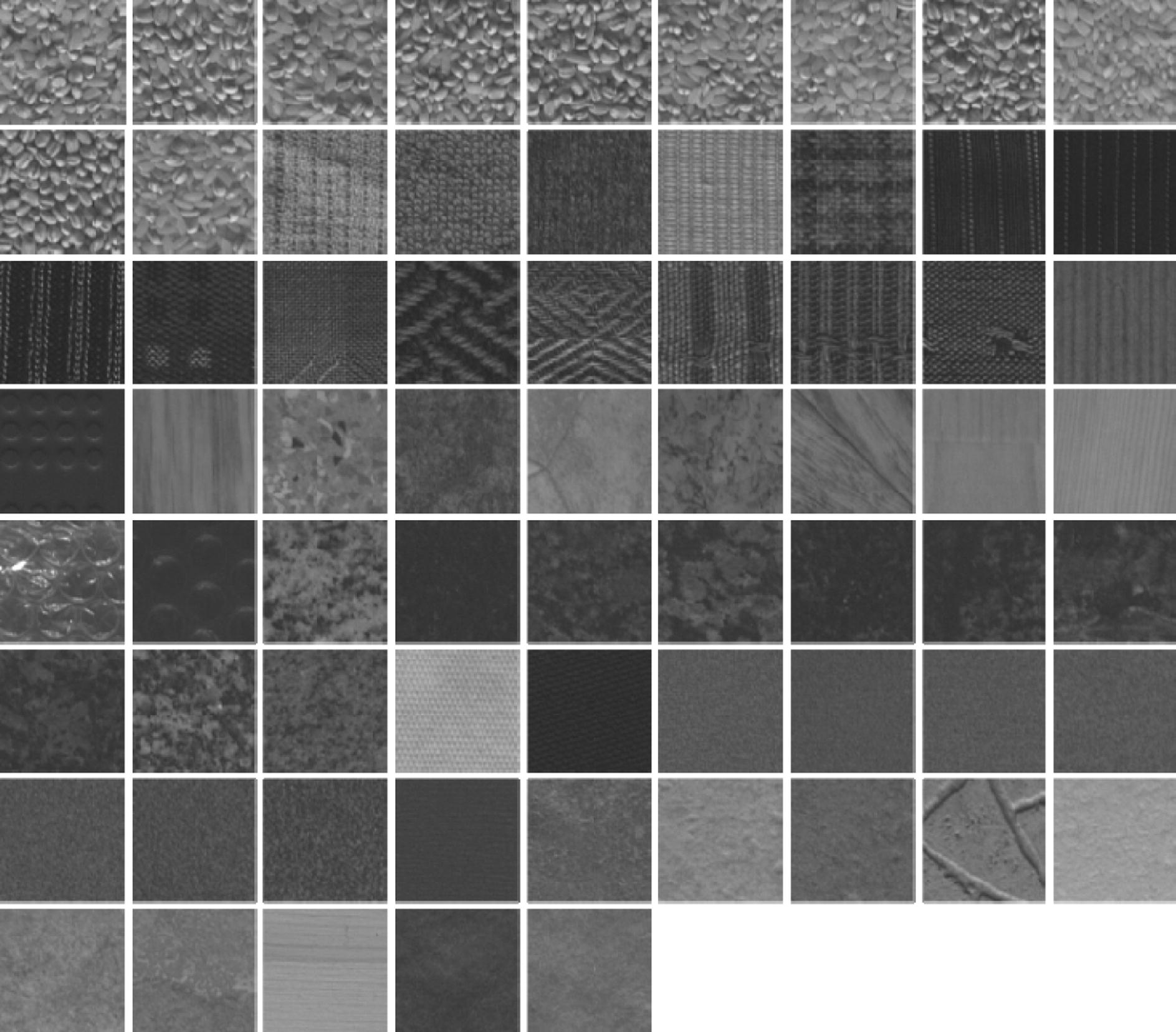
OUTEX TC 00013 dataset, 68 classes, (Fernández et al., 2012; Ojala et al., 2002).
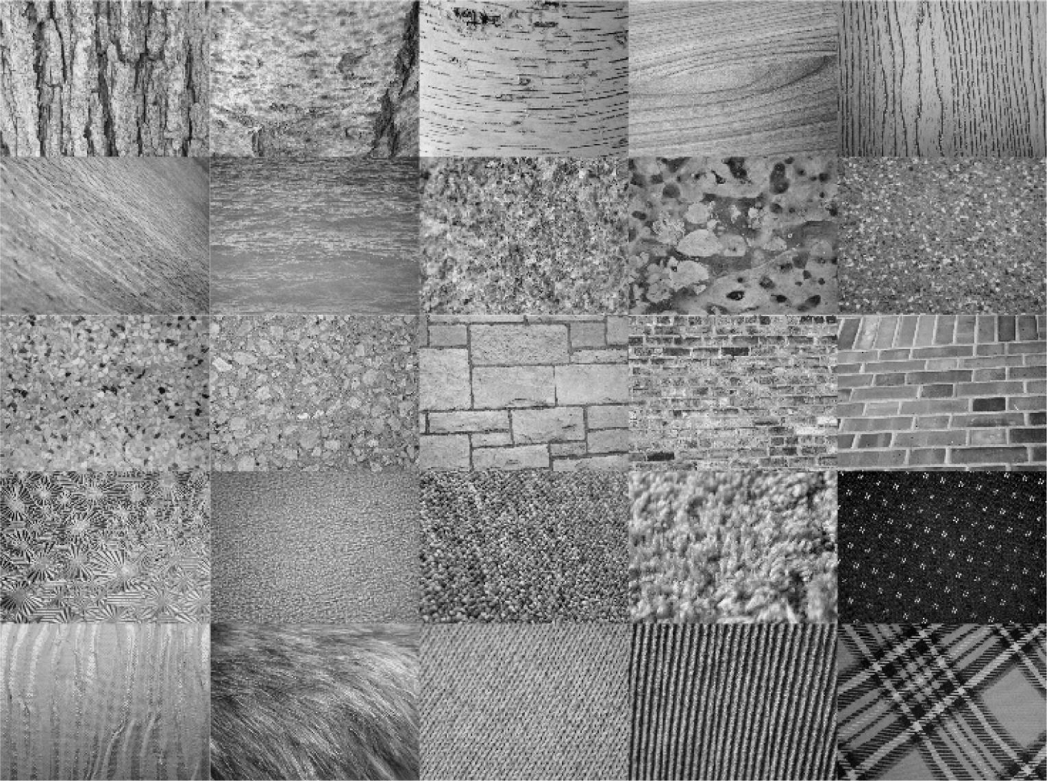
UIUCTex dataset, 25 classes, (Fernández et al., 2012; Lazebnik et al., 2005).
5 Experiments
As performance indicators we used the accuracy and the statistical rank (RK), as testing protocol the 10-fold cross validation is used. RK reports the relative position of a method against the other tested: the average rank is the most stable indicator of average performance on different datasets, it is calculated using the Friedman’s test (alpha = 0.05) applying the Holm post hoc procedure (Ulaş et al., 2012).
In the first test, Table 2, we report (using our testing protocol) the performance of well known texture descriptors (using the same parameter configuration proposed in Fernández et al. (2012)):
LBP, local binary patterns (Ojala et al., 2002);
LTP, local ternary patterns (Rahtu et al., 2012),
CLBP, completed local binary patterns (Guo et al., 2010),
ILTP, improved local ternary patterns (Nanni et al., 2010).
| Accuracy | Dataset | ||||||||
|---|---|---|---|---|---|---|---|---|---|
| Classifier | Descriptor | BO | BR | KT | MM | O0 | O1 | O3 | UI |
| SVM | LBP | 95.80 | 100 | 100 | 85.58 | 98.25 | 98.60 | 79.30 | 92.02 |
| LTP | 99.00 | 100 | 100 | 90.15 | 99.00 | 98.95 | 80.25 | 93.10 | |
| CLBP | 99.18 | 100 | 100 | 92.05 | 99.05 | 99.01 | 83.56 | 93.40 | |
| ILTP | 99.00 | 100 | 100 | 91.56 | 99.05 | 99.12 | 82.20 | 92.58 | |
| BP | LBP | 91.35 | 100 | 100 | 82.52 | 97.28 | 97.33 | 75.94 | 88.01 |
| LTP | 96.05 | 100 | 100 | 86.89 | 98.27 | 98.08 | 77.70 | 90.75 | |
| CLBP | 94.39 | 100 | 100 | 88.63 | 98.80 | 98.67 | 81.38 | 89.06 | |
| ILTP | 96.06 | 100 | 100 | 87.00 | 98.29 | 98.93 | 79.70 | 89.13 | |
Moreover we compare the performance of SVM and back-propagation neural networks (BP). We have run different configurations of BP varying the number of hidden nodes (from 3 to 11) and only the best result in each dataset is reported. For SVM we have tested radial basis function and linear kernel, the parameters setting is performed in each dataset. To select the parameters an internal 10-fold cross validation is performed using the training data (so the test set is blind).
It is clear that SVM drastically outperforms BP (as expected from the literature) and that standard texture descriptor works worse than MLQP/MLPQ3 (see next Table 3) as already shown in Paci et al. (2012).
Accuracy
Dataset
RK
Descriptor
Classifier
BO
BR
KT
MM
O0
O1
O3
UI
MLQP
SVM
99.38
100
100
93.91
99.38
99.15
86.62
96.00
5.31
GPC
99.70
99.90
100
94.19
99.13
99.05
83.82
93.93
6.50
SVM + GPC
99.88
100
100
94.14
99.13
99.01
83.82
94.13
5.62
MLPQ3
SVM
99.50
100
98.00
93.96
99.92
99.86
86.62
91.73
5.00
GPC
99.38
100
95.00
93.28
99.96
99.86
83.82
91.47
6.43
SVM + GPC
99.12
100
98.00
93.91
99.96
99.86
85.00
91.53
5.50
LPQ
SVM
99.88
100
98.50
91.41
99.92
99.86
86.62
85.93
5.44
GPC
99.88
100
88.00
91.04
99.96
99.81
84.56
86.73
6.56
SVM + GPC
99.75
100
97.00
90.87
99.96
99.81
84.71
86.93
6.43
MLQP + MLPQ3
SVM + GPC
99.95
100
100
96.56
99.96
99.86
88.09
96.80
2.19
In the following table we compare the results obtained with our texture descriptors coupled with different classifier systems:
-
SVM, SVM where the parameters (also the kernels) are optimized separately in each dataset (internal 10-fold cross validation is performed using the training data);
-
GPC, Gaussian process classifier;
-
SVM + GPC, fusion by the sum rule between linear SVM and GPC, we have used in each dataset the linear SVM (instead to optimize the kernel) for avoiding any risk of overfitting and for showing that the proposed heterogeneous system works very well also without a careful parameters tuning.
From the results reported in the previous table we can draw the following observations:
-
MLQP + MLPQ3/SVM + GPC clearly outperforms all the other methods, moreover we want to stress that this method has no parameters (we use linear support vector machine) tuned separately in each dataset.
-
SVM slightly outperforms GPC, anyway notice that we use the same parameters in all the tested datasets when we use GPC (due to execution time), while for SVM the parameters and the kernels are selected separately in each dataset.
-
MLPQ3 largely outperforms LPQ in two datasets (MM and UI), in the other datasets it obtains performance similar to standard LPQ.
| LBP | LTP | LPQ | MLQP | MLPQ3 | MLQP + MLPQ3 | ||
|---|---|---|---|---|---|---|---|
| Seconds/image | Core Duo P8600 | 0.10 | 0.30 | 0.11 | 19.25 | 1.12 | 20.37 |
| i7-2600 | 0.015 | 0.19 | 0.020 | 2.20 | 0.24 | 2.44 |
The main drawback of the proposed fusion is the execution time, making it not suited for real time applications. Anyway it is interesting to note the reduction of the execution time using a modern PC. An i7-2600 (launch date Q1-2011) is ∼10x speedier than an older Core Duo P8600 (launch date Q3-2008) and classifies an image in ∼2.5 s (notice that the execution time of SVM and GPC for classifying an image, i.e. after the training of SVM and GPC, is negligible. So in our opinion, the proposed fusion could be used in near real time applications in few years.
6 Conclusions
In this paper, we have presented an empirical study where different feature extraction approaches for texture description are compared and combined. Moreover, a configuration based on two classifiers (SVM and GPC) and two texture descriptors (MLPQ3 and MLQP) is proposed and evaluated.
Our experiments produced a number of statistically robust results regarding the generality and robustness of our system across an extensive evaluation of different datasets. The main conclusions possible to draw from the results are: (i) our proposed ensemble works well on all the tested datasets and would thus be very useful for practitioners and (ii) GPC obtains the performance only slightly lower than SVM without a careful parameters tuning.
To further improve the performance of our methods, we plan on testing more classification approaches and to compare several descriptors.
Finally we want to stress that all the code here used is open source MATLAB code so it is easy for other researchers to use/test our proposed methods. The code is available at:
-
Texture descriptors, bias.csr.unibo.it/nanni/TernaryCoding.rar;
References
- Bianconi, F., Fernández, A., González, E., Ribas, F., 2007. Texture classification through combination of sequential colour texture classifiers. In: Proceedings of the Congress on Pattern Recognition 12th Iberoamerican Conference on Progress in Pattern Recognition, Image Analysis and Applications, Springer-Verlag, Berlin, Heidelberg, pp. 231–240.
- An Introduction to Support Vector Machines and Other Kernel-based Learning Methods (1st ed.). Cambridge University Press; 2000.
- Evaluation of robustness against rotation of LBP, CCR and ILBP features in granite texture classification. Machine Vision and Applications. 2011;22(6):913-926.
- [Google Scholar]
- Texture description through histograms of equivalent patterns. Journal of Mathematical Imaging and Vision 2012
- [Google Scholar]
- Fu, X., Wei, W., 2008. Centralized binary patterns embedded with image euclidean distance for facial expression recognition. In: Proceedings of the 2008 Fourth International Conference on Natural Computation – Volume 04. Washington, DC, USA: IEEE Computer Society; pp. 115–119.
- A completed modeling of local binary pattern operator for texture classification. IEEE Transactions on Image Processing. 2010;19(6):1657-1663.
- [Google Scholar]
- Statistical and structural approaches to texture. Proceedings of the IEEE. 1979;67(5):786-804.
- [Google Scholar]
- Textural features for image classification. IEEE Transactions on Systems, Man, and Cybernetics. 1973;3:610-621.
- [Google Scholar]
- Cloth animation and rendering. In: Proceedings of Eurographics 2002 Tutorials. The Eurographics Association; 2002.
- [Google Scholar]
- Textural properties for pattern recognition. In: Lipkin B., Rosenfeld A., eds. Picture Processing and Psychopictorics Psychopictorics. New York: Academic Press; 1969. p. :347-370.
- [Google Scholar]
- On the significance of real-world conditions for material classification. ECCV (4):253-266.
- [Google Scholar]
- Texture unit, texture spectrum, and texture analysis. IEEE Transactions on Geoscience and Remote Sensing. 1990;28(4):509-512.
- [Google Scholar]
- Combining Pattern Classifiers. Methods and Algorithms. Wiley Interscience; 2004.
- A quasi-statistical approach to digital binary image representation. Revista Mexicana de Fisica. 1996;42(1):104-116.
- [Google Scholar]
- A sparse texture representation using local affine regions. IEEE Transactions on Pattern Analysis and Machine Intelligence. 2005;27:1265-1278.
- [Google Scholar]
- LibSVM guide <http://www.csie.ntu.edu.tw/∼cjlin/papers/guide/guide.pdf>.
- Local binary patterns variants as texture descriptors for medical image analysis. Artificial Intelligence in Medicine. 2010;49(2):117-125.
- [Google Scholar]
- Multiresolution gray-scale and rotation invariant texture classification with local binary patterns. IEEE Transactions Pattern Analysis and Machine Intelligence. 2002;24(7):971-987.
- [Google Scholar]
- Non-binary coding for texture descriptors in sub-cellular and stem cell image classification. Current Bioinformatics 2012
- [Google Scholar]
- Patel, D., Stonham, T.J., 1991. A single layer neural network for texture discrimination. In: IEEE International Symposium on Circuits and Systems, vol. 5, pp. 2656–2660.
- Local phase quantization for blur-insensitive image analysis. Image and Vision Computing. 2012;30(8):501-512.
- [Google Scholar]
- Gaussian Processes for Machine Learning. The MIT Press; 2006.
- Image segmentation and feature extraction. IEEE Transactions on Systems, Man and Cybernetics. 1978;75(4):237-247.
- [Google Scholar]
- Textural features corresponding to visual perception. IEEE Transactions on Systems, Man and Cybernetics. 1978;8(6):460-473.
- [Google Scholar]
- Enhanced local texture feature sets for face recognition under difficult lighting conditions. IEEE Transactions on Image Processing. 2010;19(6):1635-1650.
- [Google Scholar]
- Texture analysis. In: Chen C.H., Pau L.F., Wang P.S.P., eds. The Handbook of Pattern Recognition and Computer Vision. World Scientific Publishing Co.; 1998. p. :207-248.
- [Google Scholar]
- Cost-conscious comparison of supervised learning algorithms over multiple data sets. Pattern Recognition. 2012;45(4):1772-1781.
- [Google Scholar]
- The USC-SIPI image database [Internet]. Available from: <http://sipi.usc.edu/database>.
- The Nature of Statistical Learning Theory. New York, NY, USA: Springer-Verlag New York, Inc.; 1995.
- Automated Marsh-like classification of celiac disease in children using local texture operators. Computers in Biology and Medicine. 2011;41(6):313-325.
- [Google Scholar]
- A galaxy of texture features. In: Mirmehdi M., Xie X., Suri J., eds. Handbook of Texture Analysis. Imperial College Press; 2008. p. :375-406.
- [Google Scholar]
- Comparison of gray-level reduction and different texture spectrum encoding methods for land-use classification using a panchromatic ikonos image. Photogrammetric Engineering and Remote Sensing. 2003;69(5):529-536.
- [Google Scholar]
- Zabih, R., Woodfil, J., 1994. Non-parametric local transforms for computing visual correspondence. In: Proceedings of the third European Conference on Computer Vision (ECCV 1994). pp. 151–158.


