Yield and fiber quality traits of cotton (Gossypium hirsutum L.) cultivars analyzed by biplot method

1 Introduction

Cotton (Gossypium hirsutum L.) is one of the most extensively used textile raw materials around the world. Cotton plays a significant economic role in global economy because of its widespread use in textile industry, and provision of job opportunities in the countries where it is grown (Khan, 2013). Fiber produced by cotton serves as a raw material for the textile, seeds for oil extraction, and seed cake is utilized in the feed industries. Similarly, the stalks are utilized in the paper industry; thus, it is used for various purposes. The global population increase is also raising the demands for cotton production (Sarwar at al., 2021). The increase in global population and living standards have increased the importance of cotton. Turkey ranks 6th globally in terms of cotton production (815.000 tons annual production), and 4th in terms of cotton consumption after China, India, and Pakistan (Çoban et al., 2016).

Increasing the income from the unit area is necessary for sustainability of cotton farming. Sustainable cotton production might benefit from increased yield per acre, improved fiber quality, lower production costs, and farmer-friendly support policies. Fiber quality traits such as color and micronaire are readily affected by environmental conditions and breeding techniques compared with the genetic structure of cotton cultivars (Gul et al., 2014). Similarly, fiber length is also affected by adverse environmental conditions during boll formation phase (Pretorius et al., 2015).

Restricted cotton cultivation areas and ongoing increase in cotton consumption necessitated that cotton output should be enhanced. This requires farmers to produce higher quantity and quality from the unit area. The genetic potential of cultivars, environmental factors, and production methods influence the product's quantity and quality. Regardless of a variety's potential, environmental factors will have a significant impact on the quantity and quality of the crop produce. A variety that is successful in one location will not be able to retain the same productivity or quality features in a different location or under changing environmental circumstances (Yuksekkaya, 2002).

All breeding programs strive to produce cultivars with high yield and quality potential while exhibiting minimal variation in different environments. It is crucial to concentrate on the selection of stable genotypes that interact less with their growing environment to accomplish this aim. Since stability or minimum interaction with the environment is a genetic trait, studies may be planned to select the stable genotypes. Selection of the varieties with higher stability would help in sustainable production over large areas (Baloch et al., 2015; Orawu et al., 2017).

The assessments of quality heavily rely on interactions, which are the link between genotypes and various environmental variables. If a cultivar exhibits significant genotype × environment, genotype × years, and genotype × environment × years interactions, it is impossible to measure the genetic variation accurately, leading to inaccurate assessments. When more than one variety is tested and compared at different locations, there are differences in the ranking of quality criteria at each location. In addition to the qualitative performance of the variety, it is essential to determine if the variety is stable in terms of quality (Gul et al., 2016).

Since cotton yield, yield components, and fiber quality traits are quantitatively inherited, and environmental factors exert a significant impact on these traits. Determining the general and specific adaptability of cultivars and monitoring the yield and quality performance of cultivars and candidate cultivar under various environmental circumstances is one of the crucial phases of plant breeding (Iqbal et al., 2018). Stability is characterized as the general adaptability of a genotype, which demonstrates strong performance under diverse environments. On the other hand, special adaptability is defined as good performance in a single environment (Ali et al., 2017).

Stability is significantly affected by environmental conditions and characteristics of genotypes. Therefore, researchers use a wide variety of approaches to uncover the influence of genotype, environment, and the interplay of these two factors on stability. Genotype by environment (GE) analysis is one such method since it provides a means of quantifying and visualizing GE, which is crucial for the development of variety (Mukoyi et al., 2018; Peixoto et al., 2022). The GE interaction has a significant effect on genetic characteristics of genotypes and used for the evaluation of superior varieties (van Eeuwijk, et al., 2016; Li et al., 2017). The GGE biplot model is highly suitable for identifying environmental groups, ideal environments, and best genotypes for the most suitable environment; This method has been used by several researchers to reveal the effect of GE interaction in different plant species (Farias et al., 2016). However, it has not been applied to upland cotton in Turkey. The evaluation of test locations requires integrating the genotype (G) effect with genotype by environment interaction (GEI) as in GGE biplot method (Yan, 2001; Hu et al., 2014). For this reason, GGE biplot is used to identify the effect of variety, location, and their interactions on the stability of the tested genotypes.

The major objective of this study was to determine GE interaction among yield and fiber quality traits of three cotton cultivars at five different locations. It was hypothesized that the cultivars will exhibit significant GE interactions. The results of the study will help to select the stable cultivars for different locations based on GE biplot analysis.

2 Materials and methods

This study was conducted during 2019, 2020, and 2021 at five locations (Tepe, Boztepe, Bozçalı, Köseli and GAP International Agricultural Research and Training Center) in the southeastern Anatolia region, Turkey where cotton is intensively produced. Three commercial common cultivars (i.e., ‘DP396′, ‘BA440′ and ‘TYS 415′) were included in the study. The background information on the experimental sites are given in Table 1. The longer-term average climate data of the studied locations and weather attributes during the experimental period are given in Table 2. The soil properties of the experimental sites are given in Tables 3 and 4.

The experiment was conducted at Boztepe and GAP International Agricultural Research and Training Center Diyarbakır during 2019, Tepe and Köseli during 2020, and Bozçalı locations in 2021. Deep ploughing and herbicide application was done during November of each year. In all years, cotton received 5–6 irrigations by drip irrigation method. Based on the soil analysis, 310 kg diammonium phosphate (DAP 18–46-0) kg/ha, 90 kg potassium sulfate (51% K₂O), 30 kg magnesium sulfate (15% MgO), 330 kg/ha ammonium sulphate (21% N) before first irrigation and 500 kg/ha ammonium sulphate (21% N) were applied during flowering and boll formation periods. The study was carried out under farmer conditions with 10 plant-to-plant spacing, and 70 cm row-to-row spacing. Sowing was done on 15.04.2019, 05.04.2020 and 10.04.2021. Sampling was done on 19.10.2019, 20.10.2020 and 03.10.2021.

The study was carried out under farmer conditions with random plant selection form 30 ha. The plants with all their bolls opened were selected from an area of ​​1 m². All bolls in each position of woody and fruiting branches were collected and bagged separately. The yield and quality values ​​of the bolls in each position were weighed separately and the fiber quality parameters were measured in the HVI 1000 analyzer.

Moreover, seed cotton yield (YLD), fiber yield (FYLD), number bolls per plant (NCoc), hundred seed weight (HGW), ginning percentage (GP), fiber fineness (FF), fiber length (FL), fiber strength (FSK), and fiber elongation (ELG) were recorded for each cultivar.

2.1

2.1 Statistical analysis (GT, ET, and YT)

The collected data were analyzed by GT biplot method as recommended by Yan and Thinker (2005). The yield-trait interactions were calculated based on mean of locations and years. Biplot analyses were performed using Genstat version 14. The data were visualized for the interpretation of GT (genotype × trait), ET (environment × trait) and YT (yield × trait) using the GGE biplot software. The Fig. 1 was produced based on the performance of each genotype for each trait (GT). Similarly, Fig. 2 was generated based on the performance of environments by traits (ET) and Fig. 3 was generated based on years by traits (YT).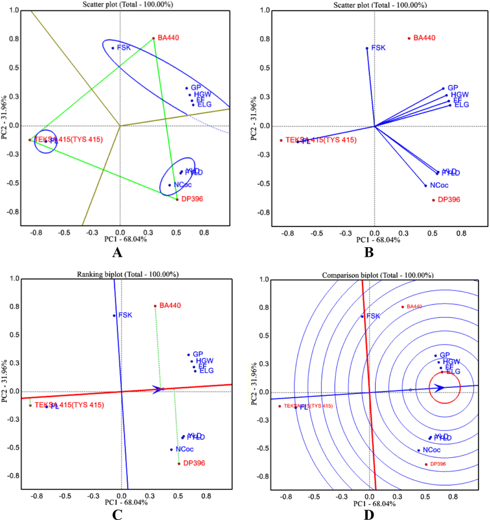

Close

Fig. 1

Genotype by trait interactions of cotton cultivars (A) locations by years, (B) which-won-where/what, (C) stability across years and (D) years and locations. Here, NCoc = number of bolls per plant, YLD = seed cotton yield, FYLD = fiber yield, HSW = hundred seed weight, GP = ginning percentage, FF = fiber fineness, FL = fiber length, FSK = fiber strength (%), ELG = elongation.

Export to PPT

Close

Fig. 2

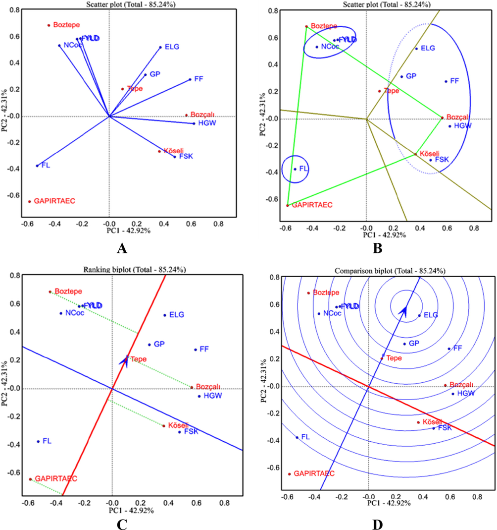
Environment by trait (ET) biplots across years (A) ET across years, (B) which-won-where of ET across years, (C) ranking biplot of ET across years and (D) comparison biplot of ET across years. Here, NCoc = number of bolls per plant, YLD = seed cotton yield, FYLD = fiber yield, HSW = hundred seed weight, GP = ginning percentage, FF = fiber fineness, FL = fiber length, FSK = fiber strength (%), ELG = elongation.

Export to PPT

Close

Fig. 3

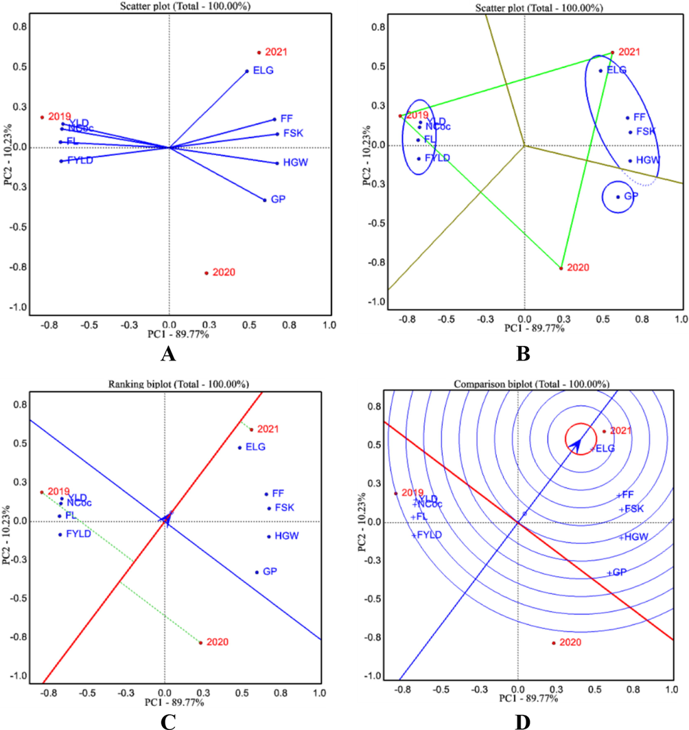
Year by trait (YT) biplot across different locations (A) relation of YT across environments (B) which-won-where of YT across environments (C) ranking biplot of YT across environments and (D) comparison biplot of YT across environments. Here, NCoc = number of bolls per plant, YLD = seed cotton yield, FYLD = fiber yield, HSW = hundred seed weight, GP = ginning percentage, FF = fiber fineness, FL = fiber length, FSK = fiber strength (%), ELG = elongation.

Export to PPT

3 Results

The mean data for yield and fiber quality traits of three cotton cultivars across five locations are show in Table 5. The pair-wise correlation of genotype by environment × traits are show in Table 6. These data were used to generate a GT biplot (Fig. 1), ET biplot (Fig. 2) and YT biplot (Fig. 3). In the GT biplot model, PC1 accounted for 68.04% of the variation, whereas PC2 represented 31.96 collectively explaining 100% of the variation. Similarly, in ET biplot model, PC1 accounted for 42.92% of the variation, while PC2 explained 42.31 of the variation making a total 85.24%. Likewise, PC1 of YT biplot model explained 89.77% of the variation, PC2 accounted for 10.23% of the variation making a total of 85.24%. The effect of PC1 is always greater than PC2 in stability analysis. Principal component analysis is applicable in situations when a small number of components explain a substantial percentage of total variation (for example, when the top two to five components justify > 60% of total variance) or when components with eigenvalues larger than one are selected. As a consequence, components with several eigenvalues were selected for the analysis since they might account for a greater share of the total variance (Groth et al., 2013).

4 Discussion

Determination of the high-yielding varieties with the highest quality can be achieved by determining the most suitable environments. Yield and quality of many plants are affected by environmental conditions (Yan, 2014). In addition, GT, ET, and YT interactions should be clearly revealed. A realistic strategy is to see a single variety, environment or year at acceptable levels for more than one trait (Xu et al., 2017). Therefore, in recent years, many researchers evaluated genotypes based on multiple traits in different plants with GT, ET, and YT (Yan and Tinker, 2006, Kendal, 2019; Sofi et al., 2021). Since there is a negative relationship between yield and quality characteristics in cotton, and this relationship may vary depending on environmental conditions (Luo et al., 2015). Therefore, it is necessary to determine the ET and YT relationships to determine high-yielding and high-quality varieties that adapt to all environments.

In this study, tested cultivars varied depending on the multi-traits. It was noted that the cultivar ‘DP396′ produced higher YLD and FYLD and NCoc, whereas cultivar ‘BA440′ had better HSW, and other quality criteria. Likewise, ‘Teksa 450′ cultivar has better FL (Fig. 1). The varieties close to the ideal center can be used as parents and preferred more in breeding programs, while varieties far from the ideal center can reduce breeding costs by being introduced in the early period in breeding studies (Ali et al., 2018). Peixoto et al. (2022) showed that, based on the correlation, GT biplot may be thought of as a strong tool for examining the relationship between characteristics, offering a graphical depiction of the genotypes and traits studied. According to Mukoyi et al. (2018), the existence of considerable GE and the correlation of features raises the need for cotton breeding to incorporate a selection index. According to Teodoro et al. (2018), cultivars are selected by farmers for more than simply their high grain production; other traits such as FL and SFI are critical to improving quality. GT is derived from multivariate approaches since genotype performance is assessed based on various attributes, as noted by Xu et al. (2017) and Oliveira et al (2018). This enables the identification of better genotypes that include all desirable traits.

This study found that the traits vary depending on the environment. Tepe location had satisfactory results for all traits, because it was located in the center of all trait vectors. Similarly, Boztepe location has good results for YLD, FYLD and NCoc, whereas Köseli, Bozçalı and GAPIRTAEC were good for specific traits (Fig. 2). Three large environmental groups were formed depending on the environmental conditions in the current study. Mare et al. (2020) selected good varieties based on high-yield and stability under diverse environments. Ali et al. (2017) indicated the presence of the mega-environments could be confirmed by conducting experiments through several years and locations. Xu et al. (2017) noted that the distinction of mega-environments is consistent with the climatic conditions of the locations. Orawu et al. (2017) reported that mega-environment describes the separation of a crop growing area into different target zones.

In YT interaction, traits varied among years and 2019 had good for YLD, FYLD, FL and NCoc. Similarly 2021 had good results for ELG, FF, FSK, and HSW, while 2020 proved specific for GP (Fig. 3). The study indicated three mega-environments among years. Darawsheh et al. (2022) reported that year effect was two to six times greater than environment. As a result, the year effect was identified as an important source of variation in all quality traits cotton. Imtiyaz et al. (2017) determined that the variation was mostly managed by the environment followed by years and genotypes. Unay et al. (2004) reported that the differences between environments (years/locations) and genotypes are very important for yield characteristics.

Three main groups were formed in correlation among studied traits in the current study. YLD, NCoc and FYLD were in the same group and positively correlated (Table 6). The ELG, HSW, FF and GP were included in second group, and they were positively correlated. On ​​the other hand, FL and FSK were in the third group, and a direct relationship could not be determined with other traits (Figs. 1-3). Chapepa et al. (2020) discovered a substantial relationship between seed yield and the quantity of bolls per plant. The quantity of bolls per plant may also be used for indirect selection. Because it has a big and positive relationship with cotton fiber production, the number of bolls per plant has a major impact on fiber yield. It is preferable to choose types with more bolls per plant. Because of the positive relationship between this characteristic and yield, Chaudhari et al. (2017) and Pujer et al. (2014) concluded that the quantity of bolls per plant is critical to improving seed cotton output. The results of Rajeev et al. (2016) demonstrated a substantial positive association between yield and boll number. According to Nawaz et al. (2019), there was a positive relationship between fiber length and strength, with an increase in fiber length corresponding to an increase in fiber strength. Rathinavel (2018) discovered that desirable quality features such as fiber uniformity and strength were lacking.

5 Conclusion

The cultivars by traits biplot indicated that ‘DP396′ was the most stable cultivar for seed cotton yield, and ‘BA440′ for fiber quality. On the other hand, the environment by traits relationship indicated that Tepe was a better location for fiber quality and seed yield, Bozçalı for quality characteristics, and Boztepe for seed and fiber yield and number of bolls. Therefore, ‘DP396′, and ‘BA440′ can be used for higher seed cotton yield and better fiber quality, respectively in southeastern Anatolia region of Turkey.

References

- Genotype by environment and GGE-biplot analyses for seed cotton yield in upland cotton. Pak. J. Bot. 2017;49(6):2273-2283.
- [Google Scholar]
- Association and heritability analysis for yield and fibre traits in promising genotypes of cotton (Gossypium hirsutum L.) Sindh Univ. Res. J. l. 2015;47:303-306.
- Correlation and path coefficient analysis of polygenic traits of upland cotton genotypes grown in Zimbabwe. Cogent Food & Agriculture. 2020;6(1):1823594.
- Chaudhari, M., Faldu, G., & Ramani, H. J. A. I. B. 2017. Genetic variability, Correlation and Path coefficient analysis in cotton (Gossypium hirsutum L.). Adv. Biores, 8(6), 226-233.
- Çoban, M., Çiçek, S., Küçüktaban, F., Yazici, L., & Çiftçi, H. 2016. Investigation of Yield and Fiber Quality Properties of Some Cotton Hybrid. Journal of Field Crops Central Research Institute, 2016, 25 (Special issue-2):112-117, Research Article.
- Environmental and Regional Effects on Fiber Quality of Cotton Cultivated in Greece. Agronomy. 2022;12(4):943.
- Farias, F. J. C., De Carvalho, L. P., Da Silva Filho, J. L., & Teodoro, P. E. 2016. Biplot analysis of phenotypic stability in upland cotton genotypes in Mato Grosso. Genetics and Molecular Research 15 (2): gmr.15028009.
- Groth, D., Hartmann,S., Klie S. and Selbig,J. 2013. “Principal Components Analysis.” In Computational Toxicology, edited by B. Reisfeld and A.N. Mayeno, 527-547. Totowa, New Jersey, USA: Springer, Humana Press, 2013.
- Genotype by environment interaction and association of morpho-yield variables in upland cotton. J. Anim. Plant Sci.. 2014;24:262-271.
- Genotype by environment and phenotypic adaptability studies for yield and fiber variables in upland cotton. J. Anim. Plant Sci.. 2016;26(3):776-786.
- Stability analysis of candidate bollgard bt cotton (Gossypium hirsutum L.) genotypes for yield traits. International Journal of Bioscience. 2018;13:55-63.
- Comparing durum wheat cultivars with genotype×yield×trait (GYT) and genotype× trait (GT) by biplot method. Chilean Journal of Agricultural Research. 2019;79(04):512-522.
- Diallel analysis of cotton leaf curl virus (CLCuV) disease, earliness, yield and fiber traits under CLCuV infestation in upland cotton. Aust. J. Crop Sci.. 2013;7(12):1955-1966.
- Genotype by environment interactions in forest tree breeding: review of methodology and perspectives on research and application. Tree Genetics & Genomes. 2017;13(60):1-18.
- Rational regional distribution of sugarcane cultivars in China. Scientific Reports. 2015;5(1):1-10.
- Mare, M., Chapepa, B., & Mubvekeri, W. 2020. Multi-Locational Evaluation of Medium-Staple Cotton Genotypes for Seed-Cotton Yield under the Middleveld Agro-Ecological Zones of Zimbabwe.
- Implications of correlations and genotype by environment interactions among cotton traits. African Crop Science Journal. 2018;26(2):219-235.
- Nawaz, S., Ahmad Malik, T., Ahmad, F., Imran, HM. 2019. Correlation of Some Morphological Traits in Upland Cotton (G. hirsutum L.).International Journal of Scientific and Research Publications, 9(3), 144.
- Yield stability of cotton genotypes at three diverse agro-ecologies of Uganda. Journal of plant breeding and genetics. 2017;5(3):101-114.
- Peixoto, M. A., Evangelista, J. S. P. C., Coelho, I. F., Carvalho, L. P., Farias, F. J. C., Teodoro, P. E., & Bhering, L. L. 2022. Genotype selection based on multiple traits in cotton crops: The application of genotype by yield* trait biplot. Acta Scientiarum. Agronomy, 44.
- Use of the AMMI model to analyze cultivar-environment interaction in cotton under irrigation in South Africa. African Journal of Agriculture. 2015;2:76-80.
- Pujer, S., Siwach, S. S., Deshmukh, J., Sangwan, R. S. & Sangwan, O. 2014. Genetic variability, correlation and path analysis in upland cotton (Gossypium hirsutum L.). Electronic Journal of Plant Breeding, 5(2): 284-289.
- Genetic Correlation Analysis for Seed Cotton Yield in Upland Cotton (Gossypium hirsutum L.). Advances in Life Sciences 5(19) Print : ISSN. 2016;2278–3849:8385-8389.
- Rathinavel, K. 2018. Principal component analysis with quantitative traits in extant cotton varieties (Gossypium hirsutum L.) and parental lines for diversity. Current Agriculture Research Journal, 6(1), 54.
- Genetic diversity among cotton genotypes for earliness, yield and fiber quality traits using correlation, principal component and cluster analyses. Sarhad Journal of Agriculture. 2021;37(1):307-314.
- Comparative efficiency of GY* T approach over GT approach in genotypic selection in multiple trait evaluations: case study of common bean (Phaseolus vulgaris) grown under temperate Himalayan conditions. Agricultural Research 2021:1-9.
- Interrelations between agronomic and technological fiber traits in upland cotton. Acta Scientiarum. Agronomy. 2018;40(1):e39364.
- Stability analysis of upland cotton genotypes to the Aegean region in Turkey. Asian J. Plant Sci.. 2004;3:36-38.
- What should students in plant breeding know about the statistical aspects of genotype × Environment interactions. Crop Science. 2016;56(5):2119-2140.
- [CrossRef] [Google Scholar]
- GGE biplot - A windows application for graphical analysis of multi-environment trial data and other types of two-way data. Agronomy Journal. 2001;93:1111-1118.
- Biplot analysis of test sites and trait relations of soybean in Ontario. Canadian Journal Plant Science.. 2002;42:11-20.
- Cultivar evaluation and mega-environment investigation based on the GGE biplot. Crop Science. 2000;40(3):597-605.
- An integrated biplot analysis system for displaying, interpreting, and exploring genotype× environment interaction. Crop Science. 2005;45(3):1004-1016.
- Biplot analysis of multi-environment trial data: Principles and applications. Canadian journal of plant science. 2006;86(3):623-645.
- Yan, W. K. 2014. Crop variety trials: data management and analysis (ed. Yan, W.)163–186 (Wiley-Blackwell).
- Yuksekkaya, Z. 2002. Genotype x environment interaction and stability analysis in cotton variety registration trials (Doctoral dissertation, Adnan Menderes University).