Water quality assessment of shallow aquifer based on Canadian Council of Ministers of the environment index and its impact on irrigation of Mathura District, Uttar Pradesh

1 Introduction

Natural water assets are directed for countless purposes including farming, drinking, household purposes, commercial production, environmental activities and so forth. Groundwater is one of the world's most essential driving force of freshwater everywhere (Bear, 1979). Around 33% of the total population of the world is anticipated to utilize groundwater mainly for drinking purpose (Nickson et al., 2005). The two noteworthy factors for variation in provincial hydrology and water assets incorporate human affairs and natural ecological changes (Li, 2014, Al-Janabi et al. 2012). The effect of human practices on nature, especially on water reserves, unavoidably intensifies with the quick improvement of the economy and booming population of the world. Babiker et al., 2007, stated that the change in the chemistry of groundwater isn’t just identified with the region's lithology and residence time but also the water which influence with rock constituents, yet additionally noticeable contributions from the air, soil and climate, as well as from contaminated sources. The transfer of untreated discharge and excessive utilization of synthetic fertilizers has concluded that the freshwater is inadmissible for both household and agricultural purposes (Bruce and McMahon, 1996). The injurious impacts on health of different toxic wastes ( M. Naushad, et al 2019) have been revealed from numerous researches like fluoride(Chandrawanshi and Patel, 1999), pesticides, nitrate, arsenic (Bruce and McMahon, 1996), Fe and total hardness, etc. in water (Soltan, 1998). But scientist developing techniques to remove contamination of heavy metals such as Cd(II), Co(II), Cu(II), and Pb(II) (M. Naushad, 2014; Naushad, et al, 2015) With just 4% of the world's freshwater assets, India reinforces over 16% of the earth’s population (Singh, 2003). The maximum cultivated field utilizing groundwater in India spread from 6.5 million hectares in the year 1951 to 35.38 million hectares in 1993 (GWREC, 1997). Around half of the irrigated land relies on the groundwater (CWC 2006) and 60% of the cereals and other foods are irrigated from groundwater wells (Shah et al., 2000). Human health and plant growth were adversely affected by the poor quality of water (Thorne and Peterson, 1954) Groundwater exploitation has increased substantially, principally for agricultural purposes. As major areas of the nation suffers annually from low rainfall and variable surface water sources flow.

The Canadian Council of Ministers of the Environment additionally built up a WQI to rearrange the revealing of intricate and massive scale water quality information (CCME 2001). The final product of the WQI calculation is a solitary unit-less number that lies between 0 and 100. (Glozier et al., 2004; 2006) and classification is shown in Table 1.

The CCME WQI is calculated as follows. $$\mathrm{W}\mathrm{Q}\mathrm{I}=100-\left(\sqrt{\frac{{\mathrm{F}}_1^2+{\mathrm{F}}_2^2+{\mathrm{F}}_3^2}{1.732}}\right)$$

The constant, 1.732, is a scaling factor (square root of three) to ensure that the index varies between 0 and 100.where:

F1 represents Scope: this expresses the degree of water quality guidelines non-compliance all through intrigue. $$\mathrm{F}1=\left(\frac{\mathrm{N}\mathrm{o}.\mathrm{o}\mathrm{f}\mathrm{f}\mathrm{a}\mathrm{i}\mathrm{l}\mathrm{e}\mathrm{d}\mathrm{v}\mathrm{a}\mathrm{r}\mathrm{i}\mathrm{a}\mathrm{b}\mathrm{l}\mathrm{e}\mathrm{s}}{\mathrm{T}\mathrm{o}\mathrm{t}\mathrm{a}\mathrm{l}\mathrm{n}\mathrm{o}.\mathrm{o}\mathrm{f}\mathrm{v}\mathrm{a}\mathrm{r}\mathrm{i}\mathrm{a}\mathrm{b}\mathrm{l}\mathrm{e}\mathrm{s}}\right)\mathrm{X}100$$

F2 represents Frequency: This expresses the level of individual tests that doesn't meet the objectives. $$\mathrm{F}2=\left(\frac{\mathrm{N}\mathrm{o}.\mathrm{o}\mathrm{f}\mathrm{f}\mathrm{a}\mathrm{i}\mathrm{l}\mathrm{e}\mathrm{d}\mathrm{t}\mathrm{e}\mathrm{s}\mathrm{t}\mathrm{s}}{\mathrm{T}\mathrm{o}\mathrm{t}\mathrm{a}\mathrm{l}\mathrm{n}\mathrm{o}.\mathrm{o}\mathrm{f}\mathrm{t}\mathrm{e}\mathrm{s}\mathrm{t}}\right)\mathrm{X}100$$

F3 represents Amplitude: This expresses the sum by which failed test don't meet their objectives This is determined in three stages.

Step 1 - Calculation of Excursion

The excursion includes several times concentration of an individual sample which is more important than the purpose.

When the test value must not exceed the objective $$\mathrm{E}\mathrm{x}\mathrm{c}\mathrm{u}\mathrm{r}\mathrm{s}\mathrm{i}\mathrm{o}\mathrm{n}=\left(\frac{\mathrm{F}\mathrm{a}\mathrm{i}\mathrm{l}\mathrm{e}\mathrm{d}\mathrm{t}\mathrm{e}\mathrm{s}\mathrm{t}\mathrm{v}\mathrm{a}\mathrm{l}\mathrm{u}\mathrm{e}}{\mathrm{O}\mathrm{b}\mathrm{j}\mathrm{e}\mathrm{c}\mathrm{t}\mathrm{i}\mathrm{v}\mathrm{e}}\right)-1$$

When the test value must not fall below the objective: $$\mathrm{E}\mathrm{x}\mathrm{c}\mathrm{u}\mathrm{r}\mathrm{s}\mathrm{i}\mathrm{o}\mathrm{n}=\left(\frac{\mathrm{O}\mathrm{b}\mathrm{j}\mathrm{e}\mathrm{c}\mathrm{t}\mathrm{i}\mathrm{v}\mathrm{e}}{\mathrm{F}\mathrm{a}\mathrm{i}\mathrm{l}\mathrm{e}\mathrm{d}\mathrm{test}\mathrm{value}}\right)-1$$

Step 2 - Calculation of Normalized Sum of Excursions

The standardized entirety of excursions, nse, is the aggregate sum by which individual tests are out of consistence. This is determined by summing the outings of their tests from their goals and dividing by the total number of criteria (meeting objectives and those not meeting objectives). $$\mathrm{n}\mathrm{s}\mathrm{e}=\frac{{\sum }_{\mathrm{i}}^{\mathrm{n}}\mathrm{e}\mathrm{x}\mathrm{c}\mathrm{u}\mathrm{r}\mathrm{s}\mathrm{i}\mathrm{o}\mathrm{n}}{\mathrm{N}\mathrm{u}\mathrm{m}\mathrm{b}\mathrm{e}\mathrm{r}\mathrm{o}\mathrm{f}\mathrm{t}\mathrm{e}\mathrm{s}\mathrm{t}\mathrm{s}}$$

Step 3 - Calculation of F3

F3 is calculated by an asymptotic function that scales the normalized sum of the excursions from objectives to yield a range from 0 to 100. $$\mathrm{F}3=\left(\frac{\mathrm{n}\mathrm{s}\mathrm{e}}{0.01\mathrm{n}\mathrm{s}\mathrm{e}+0.01}\right)$$

Though the CCME WQI is broadly acknowledged, it experiences a few restrictions. The constraints incorporate the loss of data by consolidating a few factors to a solitary index value, the loss of data among factors, the absence of convenience of the index to various biological system types and the affectability of the outcomes to the formulation of the index (Zandbergen and Hall, 1988).

2 Study area

Mathura district is located about 130 km from south-east of Delhi in the semi-desert or gray steppe soil region of south-eastern Uttar Pradesh bordering Aligarh district on the north-eastern side. The population of Mathura district is 25.47 Lakhs. The investigated area lies within latitudes 27° 14′ and 27° 17′ and longitudes 77° 17′ and 78° 12′ and covers about 3303 sq.km (shown in Fig. 1).The mean the average monthly temperature is about 42 °C in summer and 7 °C to 26 °C in winter season (Sant Lal, 2012). The only drainage in the area is the Yamuna river which enters the city from the north and after following a meandering course is passed out of the area in the SSE direction in the Agra district.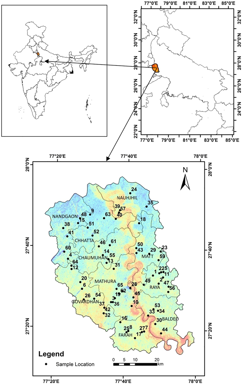

Close

Fig. 1

Base map area with sample location.

Export to PPT

3 Geology

Study area covers geological strata with the homogenous formation and does not show any significant structural complications. Quaternary alluvial tract covers most of the part in Mathura district except for few NE- SW trending ridges, which expose Delhi Super Group of rocks in the west. Heron carried out hard rock mapping (Heron, 1922); in the region, Quaternary geological and geomorphological mapping in the alluvial tract of Mathura district shown in Table 2. The Mathura Older Alluvial Plains are flat to gently undulating alluvial tract covering most of the area. In the marginal tracts of Yamuna in the southern region, badlands and ravinous tracts are developed (District & Pradesh, 2006).

4 Methodology

Geochemical data was gathered to identify the industrial impact in the Mathura district. Sixty-five water samples were taken from the piezometer borehole by the Central Ground Water Board (CGWB) from various parts of the Mathura city in July 2017. After the evacuation of this stale water, the samples were stored in prewashed high-thickness polypropylene (HDPP) bottles following the standard strategy. The groundwater samples were analyzed for pH, electric conductivity (EC), total hardness (TH) as CaCO₃, calcium (Ca²⁺), magnesium (Mg²⁺), sodium (Na⁺), potassium (K⁺), bicarbonate (HCO₃^–), chloride (Cl^–), sulphate (SO₄^2–), nitrate (NO₃^–) and fluoride (F^–), following the standard methods (APHA-AWWA-WEF 2005). Whereas EC is specified in terms of µS/cm at 25 °C. For analytical study, software’s like AquaChem and Microsoft Excel are employed by using charge-balance error for major ionic contents, did not exceed 10%.The obtained final results of major ion concentration have been compared by the Bureau of Indian Standard (BIS, 2012) and the World Health Organization (WHO, 2011)

5 Results and discussion

The vital water quality characteristics as laid down in the BIS Standards are given in Table 3 and the geochemical results are compared as illustrated in shown in Table 4.The chemical analysis of data is further analyzed for various irrigational water classification system shown in Table 5.

The variation in pH from 6.5 to 8.5is noticed in water samples. They were observed to be well within the prescribed limit. Electrical Conductivity is an estimation of the capability of fluid to convey an electrical flow. The electrical conductivity of the samples varied from 901.0 μS/cm to 14400.0 μS/cm at 25 °C. 67% of the samples show>2250 μS/cm which was above EC allowable limit. The enormous variation in EC value is associated with geochemical methods like particle exchange, reverse interaction and exchange, silicate weathering, evaporation, oxidation and sulfate reduction. (Ramesh, 2008). An increased concentration of sodium, magnesium, calcium and some other salts which result in high measures of TDS. Agrochemicals are mainly responsible and are a source for TDS as and occur as a mineral in the soil. 500 mg/L as the acceptable limit and 2000 mg/L as the permissible limit given by BIS for TDS in the absence of an alternate source of drinking water. TDS ranged from 848.0 mg/L to 17170.0 mg/L for the water samples. 78% of the water samples exceeded the 2000 mg/L permissible limit of TDS.Provenance that provides calcium incorporate feldspars from igneous and metamorphosed rocks, gypsum & carbonates (Kovalevsky et al. 2004). The value of calcium for the water samples ranged from 4.8 mg/L to 881.2 mg/L. Only 9% of the water samples exceeded the BIS permissible limit of 200 mg/L. Daily intake of sodium in excess can affect people with hypertension while pregnant ladies experience toxemia. The value of sodium varied from 45 mg/L to 2200 mg/L for the samples. A large portion of the groundwater contains generally low measures of magnesium; in any case, dolomitic rock or Mg-rich evaporitic rocks come in contact with water cause rise in value of magnesium. The value of magnesium ranged from 31.2 mg/L to 1013.0 mg/L. The permissible limit of magnesium 100 mg/L was exceeded by 84% in the water samples.The hardness of water depends upon the dissolved mineral, mostly magnesium and calcium. It does not possess a health risk. But hard water can be problematic on plumbing stopcocks, poor soap leather and detergent performance. Hardness ranged from 180 mg/L to 4720 mg/L. The allowable limit of 600 mg/L was exceeded by 69% of the samples. The value of bicarbonate varied from 39 mg/L to 1027 mg/L. 24% of the water samples exceeded this allowable limit given by BIS. It is the most widely recognized type of sulfur in extremely oxygenated water. BIS has recommended 200 mg/L as acceptable limit and 400 mg/L as the prescribed limit for sulfate. Sulfate changed from 5.1 mg/L to 2237.7 mg/L for the samples. 42% of the standards surpassed as far as possible. Youngsters, teenagers and the old are at a conceivably high danger of dehydration from diarrhea that might be caused by abnormal amounts of sulfate in drinking water (US EPA, 1999a,b). Nitrate (NO3) is found naturally in the earth and is significant for the plant as a supplement. Methemoglobinemia (blue infant disorder) in babies and is also the cause of cyanosis in infants (Young et al., 1976). The nitrate content of the samples varied from 0.01 mg/L to 149.32 mg/L. Only 12% of the samples exceeded the allowable BIS limit i.e 45 mg/L Fluoride is found in every single normal water at some concentration. Abundance in fluoride admission causes various kinds of fluorosis, basically dental fluorosis. BIS has recommended 1 mg/L as far as possible and 1.5 mg/L as permissible. All the examined samples were within the recommended limit by BIS.Taste limits for the chloride anion rely upon the related cations and are in the scope of 200–300 mg/L for sodium, potassium and calcium chloride. Given at edge, BIS has endorsed 250 mg/L as allowable limit and 1000 mg/L as the permissible limit. Chloride content for the water samples varied from 156.20 mg/L to 3905.00 mg/L. 43% of the samples exceeded the acceptable limit.

6 Water quality for irrigation

A noteworthy connection between SAR values of irrigated water and the degree to which sodium is soaked by soil. If groundwater utilized for agriculture is high in sodium concentration and low in calcium value, the cation-interchange complex may end up with sodium saturation. A low SAR of 2 to 10 demonstrates little risk from sodium; the medium risk is within 10 to 18; the great danger lies between 18 and 26 and exceptionally great danger is over 26. The lower the ionic stability of the aqueous solution, the more prominent is the sodium hazard for a given SAR value of the samples. The sodium absorption ratio for the water samples varied from 0.67 to 21.82. The sodium concentration is viewed as a crucial aspect in deciding the groundwater suitability for irrigation because soil permeability deteriorates by destroying its complex structure (Todd1980). The movement of sodium from the upper horizon to lower horizon results in hardening of the soil and prevents aeration to the roots of the plant (Wilcox, 1948). Sodium percentage for the analyzed samples varied from 8.37% to 86.66%. EC and Na % relation shown in Fig. 2.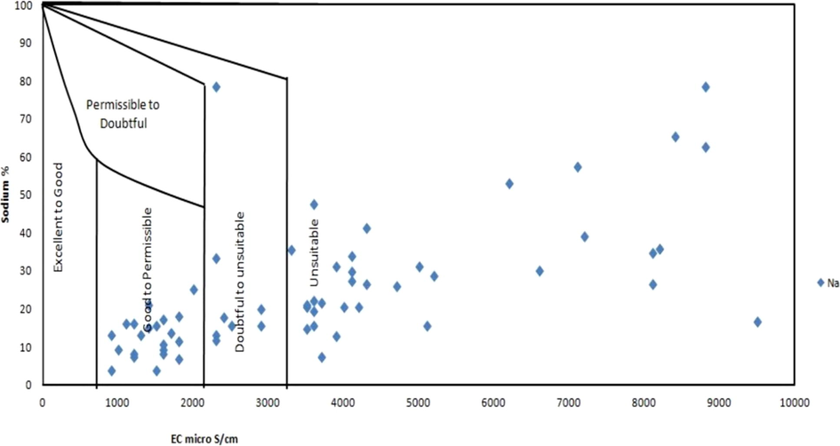

Close

Fig. 2

Relation between EC and Na % to understand water quality (Wilcox diagram).

Export to PPT

Kelley's ratio (Kelly, 1940) is obtained by sodium value divided by the Ca²⁺ and Mg²⁺ value. Excess of sodium level in waters lead to KR value more than one. Henceforth, water with a Kelley proportion under 1 are appropriate for agricultural activities, while those with a percentage more than one are unacceptable for irrigation. The values vary from 0.06 to 6.26 for the water samples. Permeability index (Doneen, 1964) has been utilized for the assurance of appropriateness for groundwater for agriculture. A continuing horticulture process will ruin the soil permeability because of Na⁺, Ca⁺, Mg²⁺ and HCO₃^– precipitation in soil. Permeability Index (PI) is an appropriate criteria for the evaluation of ions (Subramani et al., 2005). Permeability index varies from 9.59 to 98.0 for the analyzed water samples (Fig. 3). The quality of the soil is antagonistically influenced by the high magnesium content in agriculture. For this type of cases, the soil is turned out to be alkaline, bringing about diminished farming yield. The significant genesis of magnesium in the groundwater is because of ion exchange of minerals in rocks and soils by water. Magnesium hazard ranged from 45.57 to 8221.0 for the water samples. Gibbs diagram is used to illustrate factors controlling the chemistry of water. In the study area, Gibbs ratio I varies from 0.50 to 0.99 with a mean of 0.89 while Gibbs ratio II ranges from 0.28 to 0.98 with an average value of 0.71. The Gibbs ratios plotted against TDS and it is revealed that the aquifer in the study area is predominately influenced by evaporation shown in Fig. 4.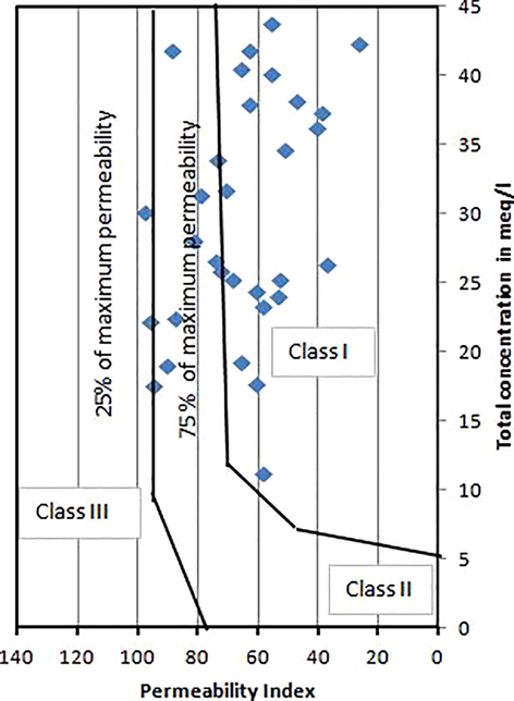

Close

Fig. 3

Evaluation of the quality of the groundwater for irrigation purposes based on PI and total ions.

Export to PPT

Close

Fig. 4

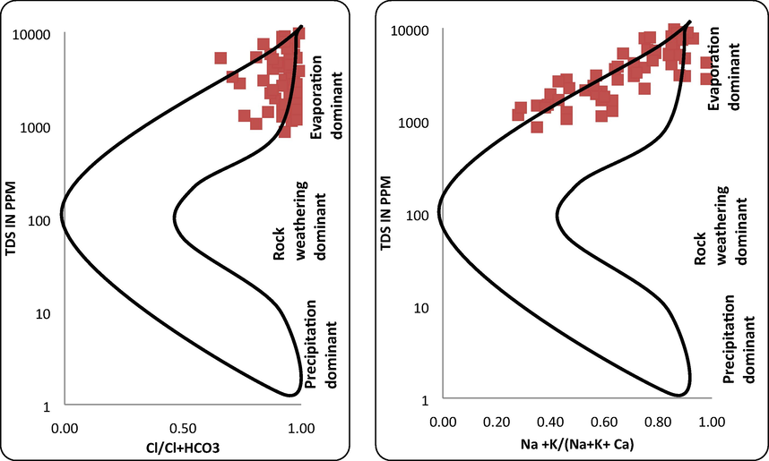
Gibbs’s diagram for the water samples.

Export to PPT

The felicity of water for farming isn't liable only on dissolvable salts is explained by Doneen (1964). Since the low dissolvability salts assemble in the soil with every continuous irrigation cycle, the dissolvable salts cause to increase the salinity in the soil. The PS of the water specimens extends from 4.58 to 112.83 meql⁻¹ with a normal of 35.11 meql⁻¹. It prescribes that the PS in the groundwater of the study area is nearly outrageous and water is unsatisfactory for utilization in farming. High sulfate content is directly proportional to the potential salinity. The overabundance entirety of carbonate and bicarbonate content in groundwater over the aggregate of calcium and magnesium substance impacts the appropriateness of water for irrigation. It very well may be deciphered that the groundwater in the investigation region indicates RSC estimation of − 90.59 to 7.71 meql⁻¹ with a standard estimation of 18.96 meql⁻¹. In light of the US Salinity Laboratory (1954), more than sixteen samples have values < 1.25 meql⁻¹ and are fine for agriculture; eleven specimens have values somewhere in the range of 1.25–2.5 meql^-1are doubtful in quality and thirteen samples have RSC values > 2.5 meql⁻¹ and are inadmissible for different activities of irrigation. Sodium carbonate accumulation is being accelerated by the water which has high RSC values and results in low fertility of soil. (Eaton 1950).

7 Water quality index

A water quality index gives beneficient techniques for complex water quality information into data that is justifiable and useable by the general population. It is prescribed that at the very least, four factors are examined, in any event, multiple times be utilized in the computation of index values. It is likewise expected that the elements and objectives picked will give applicable data about a specific site. To evaluate the appropriateness of water for different uses, there is a need to revert indices like the air quality model that will order the nature of water. WQI ranged from 1.86 to 82.25 (Table 6) for the analyzed water samples of different sample sites. The WQI map was prepared in the GIS environment using the IDW method; this map was classified on the basis CCME categorization according to their values (Fig. 5). The map having red color shows the quality of water is poor in the study region and covers the maximum area in the central part and western part of the district. A patch of blue color rises from the northern part and passes through the central part and ends at the southern area of the region shows the marginal quality of water. Yellow spots covered small area through the region and show intermediate at the northeastern part. A tiny patch of good quality water has been noticed and denotes with pink color.

Close

Fig. 5

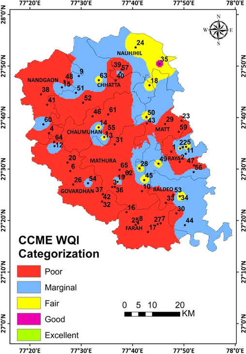
Water Quality Map based on CCME of the study region.

Export to PPT

8 Conclusion

From the results of the WQI of 65 water specimens, the quality of water in the study region lies in between poor and marginal index. Analytical techniques combined with GIS methodologies have been utilized to distinguish suitability and quality of water sites in the Mathura area for affordable drinking and agricultural purposes. The outcome of analysis demonstrate that water quality in many parts of the investigation region is unsatisfactory for household and agriculture activities. The results of physico-chemical parameters like EC, Cl^-, TDS, Ca²⁺, Mg²⁺, SO₄^2-, NO₃^– and Hardness lies above the maximum permissible limit in maximum number of samples prescribed by WHO and BIS. The suitable sites identified on the basis of the spatial distribution characteristics are located at north-east and some small area of central part of the Mathura district. The main reason for the high concentration of various water quality parameters is geogenic. Khuma, Ajai Khurd, Bazzna, Baldeo, Hasanpur, Mathura B.D.O and Bijauli are the places in the study region where the water quality was found good. Different irrigation indices show the water is not suitable for irrigation. It is proposed that appropriate treatment strategies and measures ought to be actualized before the utilization of the water for drinking and irrigation. Besides, to handle the groundwater consumption in the area, it is prescribed to adjust sprinkling irrigation for relevant usage of assets and to conquer the water scarcity faced in the future.

References

- Standard methods for the examination of Water and Wastewater, 21st edition, APHA. Washington, D.C.: AWWA & WPCF; 2005.
- Assessing groundwater quality using GIS. Water Resource Management. 2007;21:699-715.
- [Google Scholar]
- Hydraulics of groundwater. New York: McGraw-Hill International Book Co.; 1979.
- BIS 2012., Indian standard specifications for drinking water, B.S. 10500
- Shallow ground water quality beneath a major urban center: Denver, Colorado, USA. J. Hydrol.. 1996;186:129-151.
- Canadian Council of Ministers of the Environment (CCME), 2001. CCME Water Quality Index 1.0 Technical Report and User’s Manual. Canadian Environmental Quality Guidelines. Technical Subcommittee, Gatineau.
- Sant Lal, 2012. District brochure of Mathura district, U.P, Central Ground Water Board, Lucknow region, pp. 6-7.
- CWC, 2006. Water and related statistics. Central Water Commission, Ministry of Water Resources. Government of India, New Delhi, India.
- Water quality for agriculture. Department of Irrigation, University of California, Davis; 1964. p. :48.
- Water quality characteristics and trends for Banff and Jasper National Parks: 1973–2002. Saskatoon, SK, Canada: Ecological Sciences Division, Prairie and Northern Region, Environment Canada; 2004.
- Glozier, N. E., Elliot, J. A., Holliday, B., Yarotski, J., & Harker, B., 2006. Water quality characteristics and trends in a small agricultural watershed: South Tobacco Creek, Manitoba, 1992–2001. Saskatoon, SK, Ecological Sciences Division, Environment Canada.
- GSI, 2006. Final report on geoenvironmental appraisal of Mathura District, Uttar Pradesh, GSI
- GWREC, 1997. Report of ground water resource estimation committee, Ministry of water resources, Government of India, New Delhi.
- The Gwalior and Vindhyan Systems in South- Eastern. Rajputana. GSI Memoir; 1922.
- Kovalevsky V.S., Kruseman G.P., Rushton K.R., eds. Groundwater studies: an international guide for hydrogeological investigations. Pari: United Nations Educational, Scientific and Cultural Organization; 2004.
- Li, P., 2014. Research on groundwater environment under human interferences: a case study from Weining Plain, Northwest China. Ph.D. Dissertation of Chang’an University, Chang’an University, Xi’an (in Chinese).
- Surfactant assisted nano-composite cation exchanger: development, characterization and applications for the removal of toxic Pb2+ from aqueous medium. Chem. Eng. J.. 2014;235:100-108.
- Ion-exchange kinetic studies for Cd(II), Co(II), Cu(II), and Pb(II) metal ions over a composite cation exchanger. Des. Water Treat.. 2015;54:2883-2890.
- Photodegradation of toxic dye using Gum Arabic-crosslinked-poly(acrylamide)/Ni(OH)2/FeOOH nanocomposites hydrogel. J. Clean. Prod.. 2019;241:118263
- [CrossRef] [Google Scholar]
- Arsenic and other drinking water quality issues, Muzaffargarh District. Pakistan. Appl. Geochem. 2005:55-68.
- Hydrochemical studies and effect of irrigation on groundwater quality in Tondiar basin, Tamil Nadu. Anna University, Chennai, India; 2008. PhD thesis
- The Global Groundwater Situation: Overview of Opportunity and Challenges. Colombo: International Water Management Institute; 2000.
- Singh, A. K., 2003. Water resources and their availability. In: Souvenir, National Symposium on Emerging Trends in Agricultural Physics, Indian Society of Agrophysics, New Delhi, 22–24 April 2003, 18–29.
- Characterisation, classification, and evaluation of some ground water samples in upper Egypt. Chemosphere. 1998;37(4):735-745.
- Groundwater quality and its suitability for drinking and agricultural use Chithar River Basin, Tamil Nadu. India. Environ. Geol.. 2005;47:1099-1110.
- Irrigated soils. London: Constable and Company Limited; 1954.
- Groundwater hydrology. New York: Wiley; 1980.
- US EPA, 1999a. Health effects from exposure to high levels of sulfate in drinking water study. Washington, DC, US Environmental Protection Agency, Office of Water (EPA 815-R-99-001).
- US EPA, 1999b. Health effects from exposure to high levels of sulfate in drinking water workshop. Washington, DC, US Environmental Protection Agency, Office of Water (EPA 815-R-99-002).
- Guidelines for drinking water quality. Geneva: World Health Organization; 2011.
- Wilcox, L.V., 1948. The quality of water for irrigation use. US Department of Agricultural Technical Bulletin 1962, Washington.
- Prediction of future Nitrate concentration in groundwater. Groundwater. 1976;4(6):426-438.
- Analysis of the British Colombia Water quality Index forWatershed Managers: a case study of two small watersheds. Water Qual. Res. Can.. 1988;33(a):510-525.
- Assessment of Water Quality of Tigris River by using Water Quality Index (CCME -WQI) J. Al-Nahrain Univ.. 2012;15(1):119-126.