Use of non-homogeneous Poisson process for the analysis of new cases, deaths, and recoveries of COVID-19 patients: A case study of Kuwait

1 Introduction

The SARS-CoV-2 infections epidemic started in China in the last months of 2019 and has rapidly grown worldwide. On the 31st of January 2020, WHO declared an international emergency, and despite strict control, now it converted to the pandemic globally. According to the World Health Organization (WHO), this viral disease continues to emerge and presents a severe issue to public health. This pandemic also became a serious challenge and threat to the World economy (Jacobsen, 2020). According to the statistics of WHO, Worldwide, approximately 10,710,005 confirmed cases of COVID-19 pandemic caused by the SARS-CoV- 2 infection have been reported, including an estimated 517,877 deaths in approximately 216 countries (WHO, 2020). Kuwait is also one of the most affected countries by this pandemic. Around 81,573 confirmed cases of this disease throughout the country, with an estimated 519 deaths till the 25th of August 2020. The number of confirmed cases and the number of fatalities are still increasing worldwide, including Kuwait (all these counts were based on the 25th of August 2020, approximately at the end of the first layer of COVID-19 in Kuwait).

There were no available vaccines or medicine that protect against the COVID-19; therefore, several precautions were implemented in the mentioned areas and cities, and later it was implemented all over the country. In such a situation, the epidemiologists and researchers frequently utilized statistical approaches for appropriately presenting, analyzing, and forecasting the COVID-19 pandemic trends worldwide to reduce drastic effects at the early stages of its layer/wave. Several models had been used and proposed recently for the analysis of time series and point pattern data. The researchers developed various statistical techniques for analyzing and forecasting the COVID-19 situations in most affected regions and countries globally by utilizing time-series counts data (see Giuliani et al., 2020; Fanelli 2020; Yang et al., 2020).

From the previous literature, it is generally noted that in the point pattern data analysis and analyzing the rate of change, the Homogeneous and Non-Homogeneous Poisson processes (HPP and NHPP) play an essential role. For the HPP, it is to be assumed that the counting of events or patient is autonomous among dissociate regions with a homogeneous intensity, which is hardly fulfilled in real-life data. On the Other hand, for NHPP, the expected number of event occurrences and the number of patients is considered and assumed to be varied with time. Therefore, mostly the analysts prevented using HPP and preferred to use NHPP in the point pattern data analysis for both implementation time data and calendar time data (Lai and Garg, 2012). The NHPP provides a system for explaining what is measured as the point pattern data (Diggle, (2013). (Rodrigues et al., 2015) used NHPP to analyze exceedance events in air quality standards. Iervolino et al. (2014) used it to explore the intensities of earthquake ground motion. Achcar et al. (2016) and Ellahi et al. (2020) used the NHPP to analyze drought periods.

The main point that should be considered in the analysis of the number of events or patients is to determine the appropriate mean value function (m(t)) or intensity function (γ(t) = ∂m(t)/∂t) to estimate the expected number of events or patients because the NHPP has several mean value functions with different assumptions. Furthermore, to extract the significant results from the NHPPs, the most accurate values of the parameters present in the models should be determined. The previous literature (see, Ellahi et al., 2020; Achcar et al., 2016) concluded that using the Bayesian approach under MCMC simulation performed significantly in the estimation of parameters for the NHPP models. Other than these, many researchers have discussed the Bayesian approach and inference for the NHPP models with various prior distributions for the model parameters (Guarnaccia et al., 2015; Meng et al., 2017; Vicini et al., 2012).

This paper mainly analyzed confirmed cases, recoveries, and deaths of the COVID-19 first layer in Kuwait by utilizing the point processes to these counts. For this purpose, we modeled the cumulative numbers or counts of confirmed cases, recoveries, and deaths by using linear intensity functions and the power-law process in NHPP. These are the two different parametrical forms of intensity functions discussed in the analysis of accumulated numbers of drought events (Ellahi et al., 2020; Achcar et al., 2016). For the estimation of NHPPs parameters, we used the Bayesian approach with non-informative priors of model parameters under MCMC simulation and selected the appropriate models using Deviance Information Criteria (DIC). The current study explored the usefulness and significance of the presented research framework to analyze the COVID-19 new confirmed cases, recoveries, and deaths in an area. The study results will help the health organizations or authorities to develop the approaches based on the current resources and situations due to pandemics.

2 Methodology

3 Bayesian inference

This section introduced the Bayesian analysis for LIF and PLP model, and their required posterior summaries were obtained using MCMC simulations. Our interest in this analysis is to develop or find the posterior distributions of NHPP models parameters. Therefore, it is to be assumed that the parameters of the NHPP models have uninformative uniform priors, i.e., all the parameters of ϴLIF = (λ0, α) and ϴPLP = (α, β) follows U(a, b), where a and b are the hyperparameters of the prior distributions. Further, prior independence among the parameters is also assumed. Let, P(ϴLIF or ϴPLP) be the prior joint distribution of the parameters, and L(ΘLIF or ΘPLP;St) is the likelihood function of the model under study then the joint posterior distribution for the P(ϴLIF or ϴPLP /St) can be expressed as, P(ΘLIF or ΘPLP/St)∞P(ΘLIF or ΘPLP)L(ΘLIF or ΘPLP/St) where the likelihood function from the time truncated model is given by, L(ΘLIF or ΘPLP;St) (πj = 1 k γ (tj/ΘLIF or ΘPLP)) exp (-m(T/ΘLIF or ΘPLP)) where γ (tj/ΘLIF or ΘPLP) and m(T/ΘLIF or ΘPLP) are the intensity function and mean value function of LIF or PLP. The simulated samples for P(ΘLIF or ΘPLP/St) and the posterior summaries of interests for ϴLIF and ϴPLP are obtained under standard MCMC algorithm, i.e., Gibbs sampling. In MCMC, Gibbs sampling is initiated by an arbitrary value, which can be assumed or calculated from the priors and then gradually converged to a target value. Several techniques can be used to check this convergence; trace plots and some useful summary statistics are frequently used. These plots and results provide clear indications of stabilized simulations. The convergence can be evaluated with a reasonable degree of assurance by utilizing these indications. For this purpose, Su and Yajima (2012) introduced the R software library “R2jags,” which provides considerable simplification. Based on well known Bayesian adequacy measure called Deviance Information Criteria (DIC), we choose the suitable model of NHPP for modeling each study variable, i.e., the number of new confirmed cases, the number of recoveries, and deaths concerning the time interval T = 184 days. For further details of the intensity functions and Bayesian approach, kindly visit the Guarnaccia et al., 2015; Achcar et al., 2016; Meng et al., 2017 and Ellahi et al., 2020.

4 Results

Fig. 1 presents the Bar-plots for the frequency distribution of new confirmed cases, recovered cases, and deaths. Fig. 1a indicates that the ratio of the latest confirmed cases increases after the 1st of April 2020. This ratio reaches its peak in the mid of May, and after the 1st of June, the number of new confirmed cases on a daily basis moderately decreased. Fig. 1b also provides detailed information about the recoveries of SARS-CoV-2 infected patients. Its bar-plot shows that in the start of April the number of recoveries was very low concerning the new confirmed cases, but at the 1st of June 2020 ratio or the number of recoveries were much more than the new confirmed cases, i.e., the number of recoveries were approximately 1500, and the number of new cases was around 1050. However, from the mid- month of June, the number of new confirmed cases was more than the number of recovered patients on a daily basis. Fig. 1c presents that the number of deaths increases after the mid of April, and in May and June, the number of deaths is higher than the other months. However, before starting July, the number of deaths daily was reduced until the 25th of August.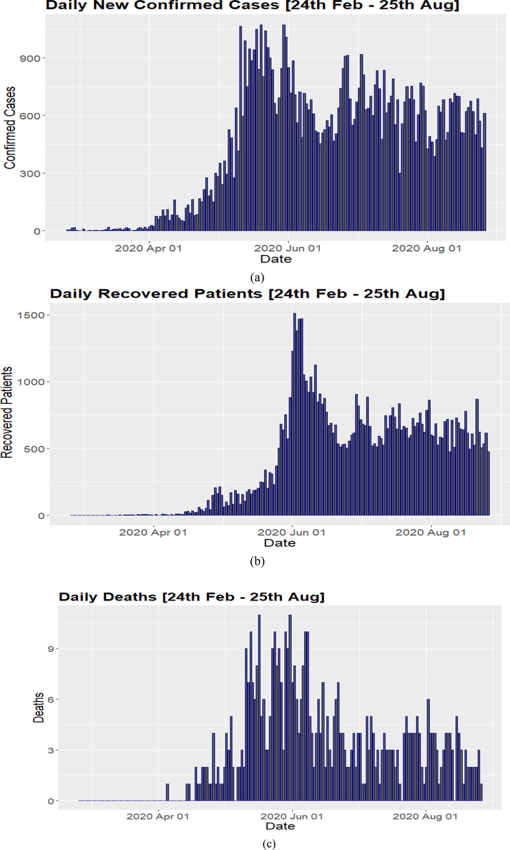

Close

Fig. 1

Bar-plots for the counts of daily new confirmed cases recoveries and deaths.

Export to PPT

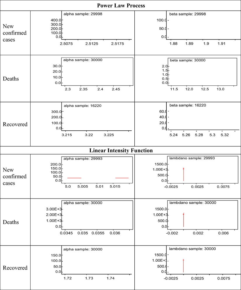
Fig. 2 shows the accumulated number of new confirmed cases, the accumulated number of recoveries and deaths with respect to time or days for the time period from the 24th of February to the 25th of August 2020. These plots present the total aggregated new confirmed cases recoveries and deaths for each day versus the days of each study month. To model the accumulated number of new confirmed cases, recoveries, and deaths, we considered the two NHPP models, i.e., PLP and LIF, and the parameters for each model and each study variable are estimated using the Bayesian approach under MCMC simulations as briefly explained in the methodology section. For prior distributions of required parameters in our study, we assumed that in the case of ΘLIF = (λ0, α), λ₀ ∼ [0,100] and α ∼ U[0,100], and in case of ΘPLP = (α,β), α ∼ U[0,100] and β ∼ U[1,100]. There is no hard and fast rule for the values of the parameters of prior distributions, i.e., for hyperparameters. Those values of hyperparameters can be used for which the distributions have minimum variance, or these values can also be considered based on the researcher's personal experiences related to concern problems. In the Bayesian analysis of each NHPP model, the above discussed non-informative uniform priors were utilized for each study variable. The single Markov chain was set up for the sample's simulations of the joint posterior distribution of LIF and PLP and sampled it for 35,000 reiterations. The first 5000 iterations were considered as the burn-in samples to eliminate or minimizes the effects of the initial value used in the iteration process. Based on history plots, we considered the number of burn-in samples, where the distributions become in equilibrium states, see Fig. 3, and the remaining 30,000 were used for the convergence checks and summarization of the results. The trace plots in Fig. 4 indicate the convergence of the MCMC, and it can be verified by the summary statistics regarding each parameter provided in Table 1. The marginal posterior density plots of all the parameters of each model for individual study variables are presented in Fig. 5. Similarly, the autocorrelation plots are also shown in Fig. 6. It provides the pattern of serial correlation in the chain, where the consecutive draws of the parameters from the conditional distributions were correlated.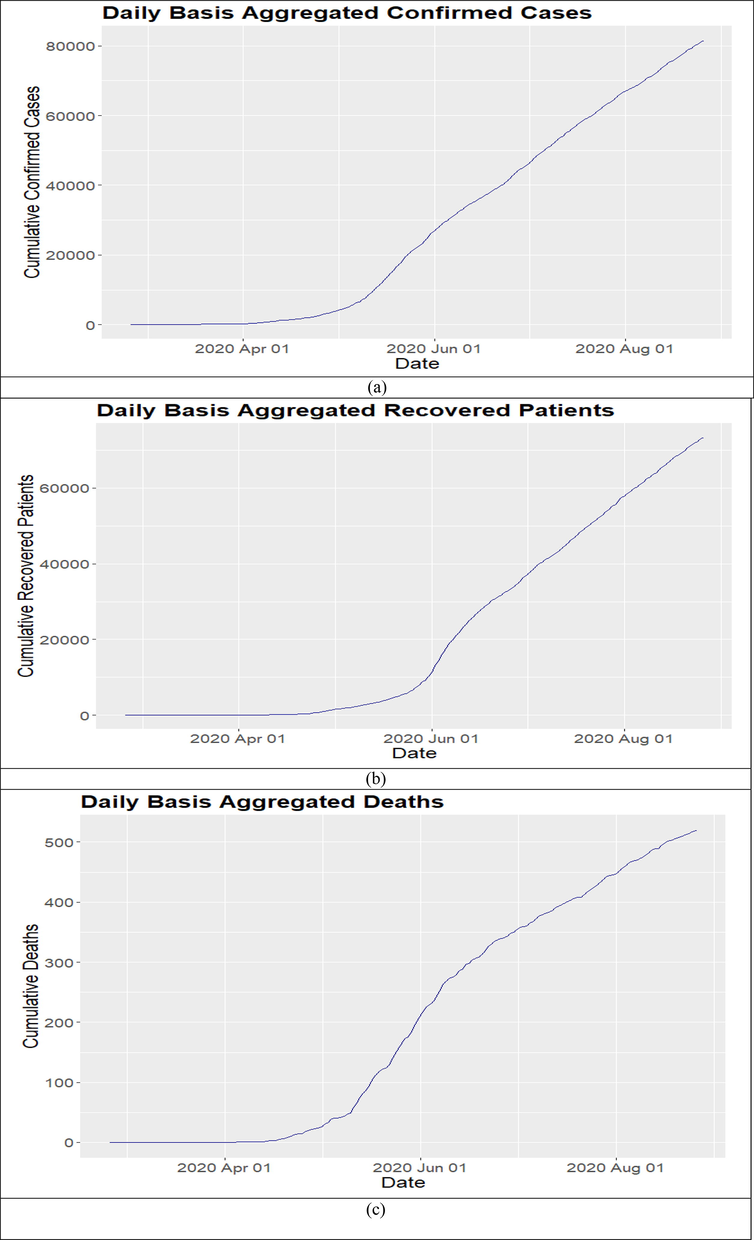

Close

Fig. 2

Accumulated numbers of new confirmed, recovered and deaths of COVID-19 patients.

Export to PPT

Close

Fig. 3

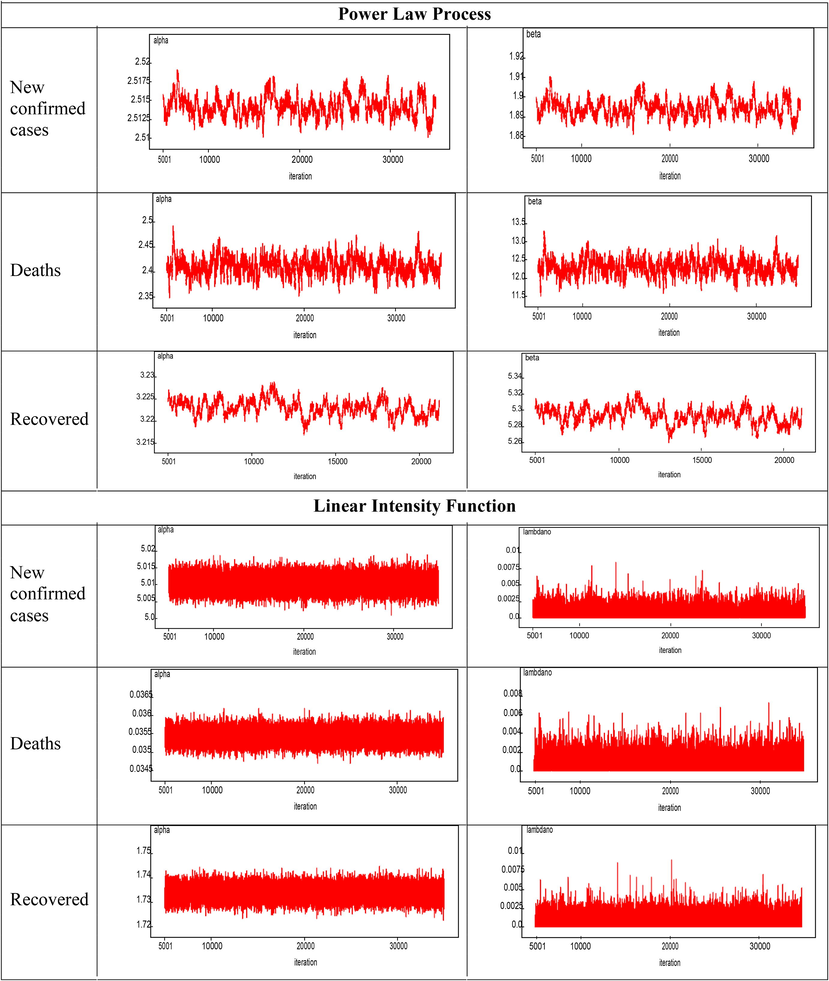
History plots for each parameter of PLP and LIF.

Export to PPT

Close

Fig. 4

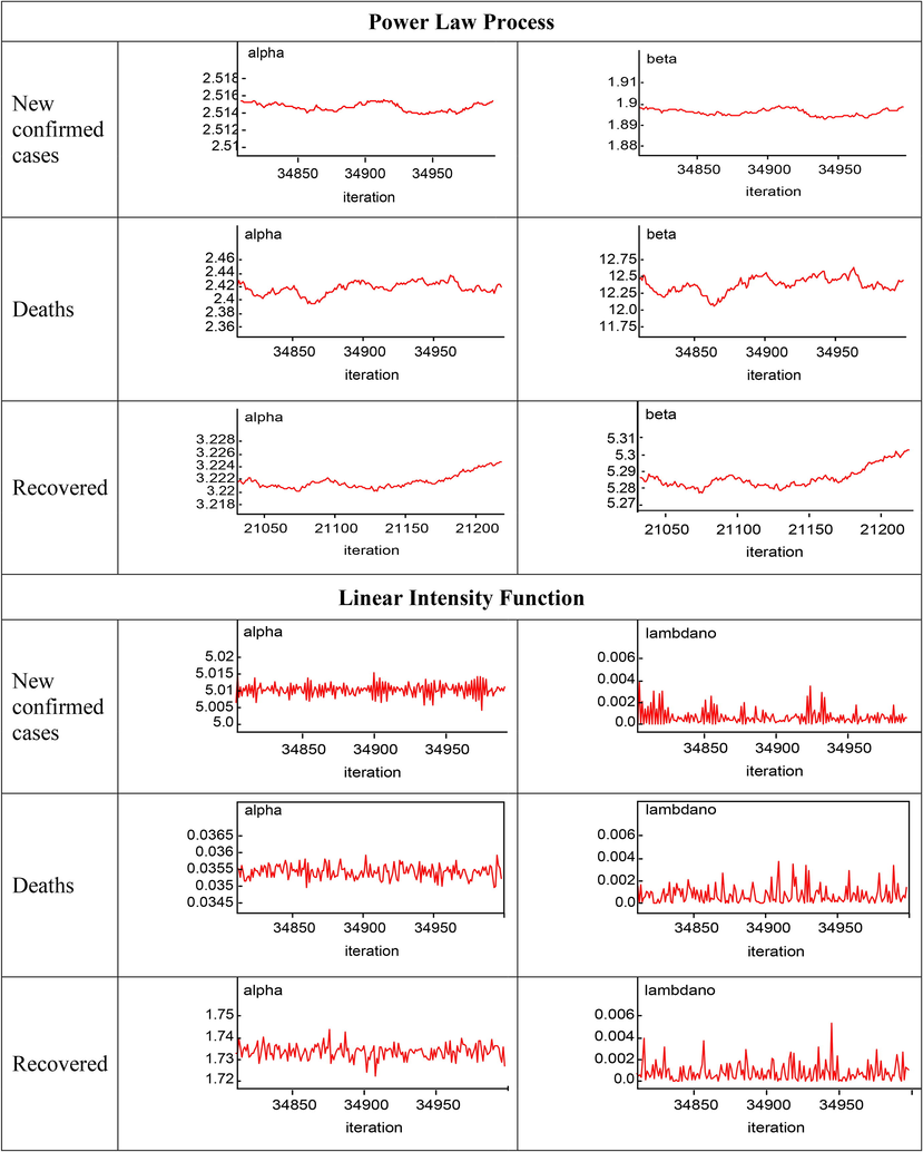
Trace plots of each parameter for PLP and LIF.

Export to PPT

Close

Fig. 5

Margional posterior density plots of each parameter for PLP and LIF.

Export to PPT

Close

Fig. 6

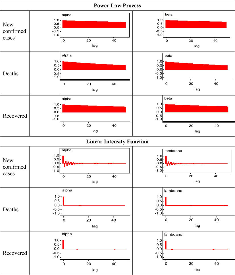
Autocorrelation plots of each parameter for PLP and LIF.

Export to PPT

The Monte Carlo estimates for the Posterior summaries of interest and the Monte Carlo errors based on 30,000 simulated samples, by taking every 150th simulated value, are given in Table 1. Similarly, the Monte Carlo measures for the DIC values of each model and each study variable are presented in Table 2. In the case of LIF, the DIC values for the new confirmed cases, deaths, and recoveries are 338338, 4608.70, and 239798. Similarly, the DIC values in the case of PLP for the new confirmed cases, fatalities, and recoveries are 279248, 4024.110, and 227896. The DIC values in the case of PLP for each study variable are much less than or smaller than the DIC values of LIS. Therefore, we selected the NHPP model based on PLP and used it for the analysis of the new confirmed cases, deaths, and recoveries regarding COVID-19. We use the marginal posterior means of the PLP parameters from Table 1 to model each study variable and estimate the accumulated counts of these study variables with respect to time. The RMSE's of the calculated results for new confirmed cases, deaths, and recoveries are 5489.937, 54.4633, 5513.525, which are also provided in Table 3. The estimated and observed number of new confirmed cases, fatalities, and recoveries are presented in the plots of Figure 7. The values of RMSE, s in Table 3 and the plots of Fig. 7 clearly show that the PLP performs very well in the estimations of COVID-19 pandemic study variables. The Redline in the plots presents the estimated accumulated means estimated at each day. The number of new confirmed cases, deaths, and recoveries of SARS-CoV-2 infected patients was reported using the estimated parameter values. Here the term accumulated denotes the mean value function assessed or evaluated at each day counts of our study variables.

Close

Fig. 7

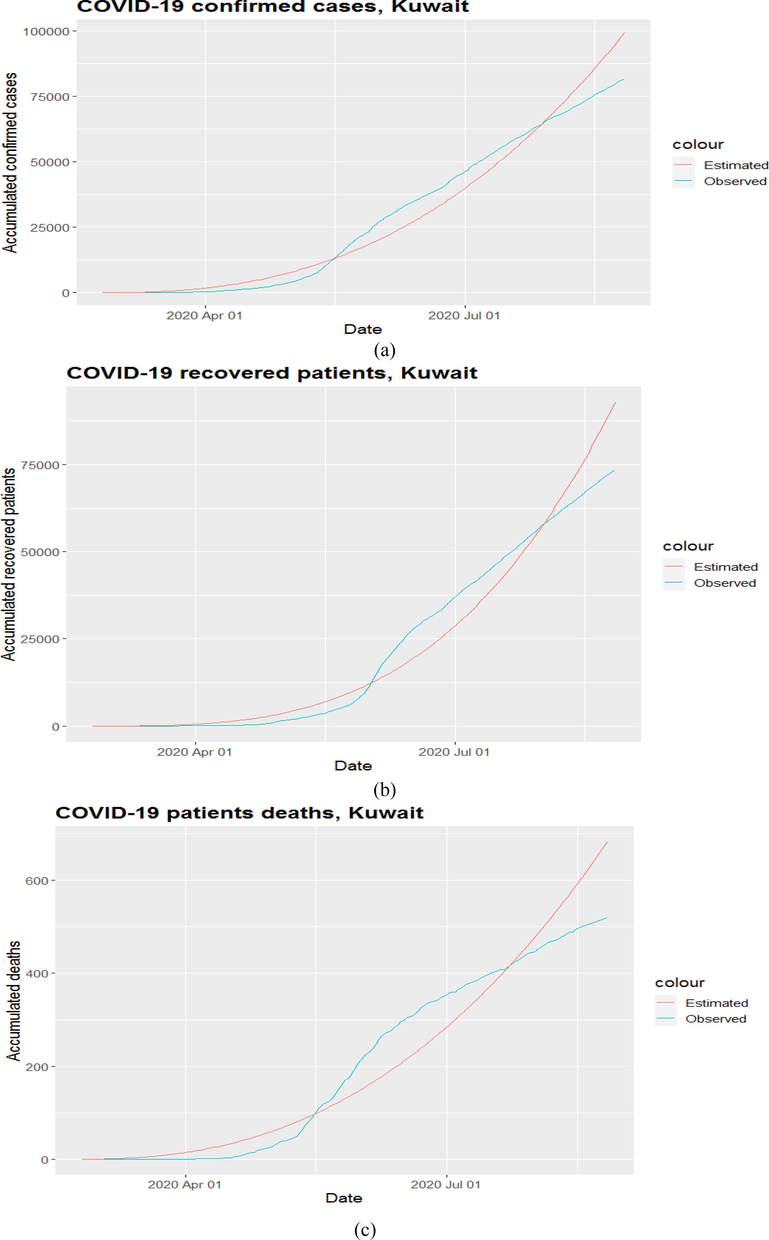
Estimated and onserved counts of daily new confirmed cases recoveries and deaths.

Export to PPT

5 Discussion

The WHO indicates that COVID-19 viral infection keeps on developing, and presenting a significant issue to Public health and the world economy. On the 31st of January 2020, WHO announced a worldwide emergency, and regardless of strict control, now it changed over to pandemics worldwide. Kuwait is also one of the most influenced countries by this pandemic. The number of affirmed cases and the number of deaths are still increasing worldwide, including in Kuwait. As the level of that infection changes state to state; thus, the executions of these controlled systems or guidelines additionally fluctuate as indicated by the national circumstances. Consequently, the utilization of statistical tools has incredible noteworthiness to anticipate or predict the pandemic patterns of this contamination around the world.

This paper uses multiple statistical tools for the descriptive and inferential analysis of COVID- 19 patients in Kuwait. At the initial stage, Bar plots and Time-series plots were used for the descriptive analysis of the number of confirmed cases, numbers of deaths, and recovered SARS-CoV-2 infected patients. Fig. 1 shows the bar plots based on the daily counts of new cases, deaths, and recoveries from the 24th of February 2020 to the 25th of August 2020. These bar plots present the fluctuations in the counts and provide a detailed summary of the study variables daily with their six-month pattern. Fig. 2 shows the time series plots for the accumulated counts of new confirmed cases, deaths, and recoveries. These plots present the rate of change of the counts concerning time. Fig. 2 (a, b, and c) indicate that the rate of change was moderately increasing from May 2020, and it became so high in June 2020 for each study variable. However, the rate of change became moderate and remained the same from the end of June till the 25th of August.

A common problem with counts data in statistical inference is the selection of an appropriate model. In our case, we also observed that the appropriate NHPP models could be of great use. Interestingly, other intensity functions can also be used similarly as considered the LIF and PLP in our study. We obtain the posterior distribution summaries of quantities of interest by using MCMC techniques under Gibbs sampling. The library R2jags of software R was very helpful in the simulation of samples from the posterior distributions of intensities parameters. These samples are then used to obtain the empirical summaries of the statistics for the selection of appropriate NHPP models and are used to draw inferences on the parameters (i.e., about the actual values of the model parameters) of interest. The convergence of Gibbs sampling techniques was monitored by MC errors (provided in Table 1) and observed by using the history plots, trace plots, posterior density plots, and autocorrelation plots, as shown in Figs. 3, 4, 5, and 6. The best models for our study variables were selected based on existing Bayesian adequacy criteria such as DIC (the approximation of Bayes factor); the lower the value of DIC better will be the model. The PLP models for the counts of new confirmed cases, deaths, and recoveries were better than the LIF, as indicated by the values of DIC in Table 2. Therefore, for our further analysis, for estimations of the counts of new cases deaths and recoveries with its behavior for the observed time interval, we utilize the PLP models.

Considering the PLP models (which are the best-fitted models), we observed from the results of Table 1, that the MC error for both parameters (alpha and beta) is low and can be acceptable, the marginal posterior standard deviation is also so small, which indicates that all the parameter values for the generated samples were concentrated at marginal posterior means of α and β in each case. As we know, the intensity function has a flexible behavior for PLP due to the value of α. The function of γ(t/ϴ)_PLP is decreasing for α less than 1, increasing for α greater than one, and constant for α = 1 (i.e., the NHPP is HPP). In our study, for the newly confirmed cases, the value of α is 2.514; for the counts of deaths, the value of α is 2.412; and for the counts of recovered patients, α is 3.223, which are greater than 1. So, in our study, the intensity function is increasing. By using these values of α and β provided in Table 1, we could find the estimated average counts of new confirmed cases, deaths, and recoveries for each specified value of time.

Fig. 7 (a, b and c) presented the estimated accumulated counts (using the results of Table 1 for PLP) of each day with the observed accumulated counts versus the days of all studied months. These plots and their respective RMSE, s provided in Table 3, clearly show the better performance of the PLP model in each case.

6 Conclusion

This paper presents the framework to analyze the accumulated counts of new confirmed cases, deaths, and recoveries of SARS-CoV-2 infected patients in Kuwait from the 24th of February 2020 to the 25th of August 2020, i.e., the first layer of COVID-19 pandemic. The descriptive analysis of the counts summarizes the data efficiently and effectively. The NHPP models with linear intensity function and Power-law process being used for comparative study of the behavior of accumulated counts of COVID-19 pandemic. The parameters of the NHPP models were computed by using a Bayesian approach with Gibbs sampling under the MCMC algorithm. That performs very well in the simulation and estimation of model parameter values. The results and graphs indicate that the NHPP models under PLP perform much better than LIF. The presented data clearly showed that during the first layer of COVID-19 Pendamic in Kuwait, the intensity varied with time and reached a high level in the mid of our study period. These fluctuations in the intensities were efficiently estimated by the appropriate estimated intensity function in NHPP. The current study explored the usefulness and significance of the presented research framework to analyze the SARS-CoV-2 new confirmed cases, recoveries, and deaths in an area. Similarly, the proposed framework may be utilized for other layers of the COVID-19 pandemic in Kuwait and other countries or regions. The outcomes of the study will support the health organizations or authorities in developing the approaches or strategies to overcome the effects of the COVID-19 pandemic dependent on the current resources and circumstances due to the pandemic. It is essential to point out that for the comparative study to improve the results, different intensity or mean value functions of NHPP models can also be utilized.

The results obtained from the proposed framework may be improved by utilizing the comparative analysis of some other suitable intensity functions or by proposing an efficient and sufficient intensity function for the NHPP model in such particular case studies. Furthermore, the proposed framework doesn't consider the abrupt change in the process, which is its drawback. These abrupt changes could be considered, and the errors in the study may be reduced by assuming a specified parametrical form consist of some additional parameters for these particular changes in the process. The work on all these limitations and the comparative studies of all COVID-19 pandemic layers in Kuwait is the aim of our future studies.

References

- D. Giuliani, M.M. Dickson, G. Espa, F. Santi, Modelling and predicting the spatio-temporal spread of coronavirus disease 2019 (COVID-19) in Italy (2020). 10.2139/ssrn.3559569.
- Analysis and forecast of COVID-19 spreading in China, Italy and France. Chaos Solitons Fractals. 2020;134:109761
- [CrossRef] [Google Scholar]
- Modified seir and ai prediction of the epidemics trend of COVID-19 in China under public health interventions. J. Thorac. Dis.. 2020;12(3):165-174.
- A detailed study of NHPP software reliability models. J. Softw.. 2012;7(6):1296-1306.
- [Google Scholar]
- A non-homogeneous Poisson model with spatial anisotropy applied to ozone data from Mexico City. Environ. Ecol. Stat.. 2015;22(2):393-422.
- Sequence-based probabilistic seismic hazard analysis. Bull. Seismol. Soc. Am.. 2014;104(2):1006-1012.
- Use of non-homogeneous Poisson process (NHPP) in presence of change-points to analyze drought periods: a case study in Brazil. Environ. Ecol. Stat.. 2016;23(3):405-419.
- Analysis of agricultural and hydrological drought periods by using non-homogeneous Poisson models: Linear intensity function. J. Atmosph. Solar-Terrest. Phys.. 2020;198:105190.
- An analysis of airport noise data using a non-homogeneous Poisson model with a change-point. Applied Acoustics. 2015;91:33-39.
- Data analysis on incomplete failure of ship electromechanical system based on bayesian method. In: 2017 Prognostics and System Health Management Conference (PHM-Harbin). IEEE; 2017. p. :1-7.
- Non-homogeneous Poisson processes applied to count data: a bayesian approach considering different prior distributions. J. Environ. Protect.. 2012;03(10):1336-1345.
- WHO, 2020. accessed on August 25, 2020. https://www.who.int/emergencies/diseases/novel-coronavirus-2019?gclid=CjwKCAjwrvv3BRAJEiwAhwOdMzEtuvWQBQPQNS8H8aLpDrfCdkilUEKk__M4leN9ezfIgMgv04cRqhoCA9wQAvD_BwE.