Ultrasound image assisted diagnosis of hydronephrosis based on CNN neural network

1 Introduction

Hydronephrosis is a common disease in the urinary system, and clinicians are looking forward to determining the cause of the disease. Moreover, the obstruction can occur anywhere in the urinary tract. The reason is the defect of the ureteropelvic junction, the obstruction of the urinary tract, or the extra-uropathic lesion (Portero et al., 2019; Muraoka et al., 2020; Misztal et al., 2020; Orts-Del’Immagine et al., 2020; Ohata et al., 2019; Kotani et al., 2019). Ultrasound detection is the main means of diagnosing hydronephrosis, but there are many kinds of interference factors in actual detection. Therefore, it is necessary to combine the auxiliary diagnosis measures to improve the diagnosis (Liu et al., 2017).

At present, renal magnetic resonance imaging (MRI) examination mainly uses 1.5 T MRI, but 3.0 T MRI has a higher signal-to-noise ratio, faster imaging and better spatial resolution (Miyan et al., 2019; Ruan et al., 2019; Gu et al., 2019; Bhrini et al., 2020; Ruan et al., 2019). Moreover, it can provide good anatomical image high contrast and sufficient image resolution, so new imaging techniques are increasingly used to evaluate renal function (Huynh et al., 2016). The current common MR examination methods include Perfusion-Weighted Imaging (PWI) (Ma et al., 2017), MR renography (Rianthavorn and Limwattana, 2015), contrast plasmapheresis (Chen et al., 2015), diffusion-weighted imaging (DWI) (Salehi et al., 2017) diffusion tensor imaging (DTI) (Zhang and Yang, 2016), blood oxygenation level-dependent (Ren et al., 2016) (BOLD) and renal sodium ion magnetic resonance imaging (Alioua et al., 2016) (sodium MRI). MR diffusion imaging is currently the only non-invasive method for quantitatively detecting the diffusion and microcirculation perfusion information of living tissue at the molecular level. The diffusion motion of molecules is derived from the random thermal motion of water molecules at the microscopic level, that is, Brownian motion, which is the basis of MR diffusion imaging (Gonzalez-Sosa et al., 2015). Clinical applications of MR diffusion imaging include MR diffusion-weighted imaging (DWI) and MR diffusion tensor imaging (DTI) (Bejar and Miranda, 2015). MR diffusion-weighted imaging (DWI) uses the microscopic random motion of water molecules in the gradient field and changes in apparent diffusion coefficient (ADC) of the renal parenchyma to assess changes in renal function, which can reflect changes in the diffusion amplitude of water molecules (Iakymchuk et al., 2015; Pluim et al., 2019; Song et al., 2018; Donatelli et al., 2018; Sarbu et al., 2020). The transport of water in renal parenchyma has an important effect on renal function. The ADC value of renal parenchyma can be affected by water content, renal perfusion and renal blood volume. Also, renal blood flow and tubule fluid flow can affect ADC value (Che et al., 2017). Foreign literature reports DWI has been used to evaluate renal function changes in a variety of kidney diseases, such as renal arteriosclerosis and kidney transplantation (Burrascano et al., 1999). MRI diffusion tensor imaging (DTI) is based on DWI to quantify the diffusion anisotropy of water molecules from multiple directions using diffusion-sensitive gradients to reflect the fine structure and functional information of living tissue. It can measure not only the ADC value but also the anisotropy index value. The latter provides a difference in the direction of dispersion of water molecules, which can provide more diagnostic information for renal function and structural changes (Zhao et al., 2016). The basis of its application is based on the radial distribution of renal tubules, which leads to anisotropy of diffusion. The renal medulla diffusion tractography (DTT) post-processing technique can display densely arranged radiation beams in the renal medulla and can visually show the tubular walking and distribution patterns (Bakhtiyari et al., 2015).

2 Material & methods

The biggest difference between convolutional neural networks and BP artificial neural networks is that adjacent neurons in the CNN structure are not fully connected, but partially connected, and the perceptual region of each neuron comes from some neurons in the upper layer of the neuron (Prandi et al., 2017).

The goal of the Super-Resolution Convolutional Neural Network (SRCNN) is to learn to obtain the mapping function F to achieve an end-to-end mapping between the low-resolution image block Y and the high-resolution image block X. Since the above operations can be realized by convolution, a convolutional neural network can be established. The network structure is as shown in Fig. 1 (Lombardo and Pizzo, 2016).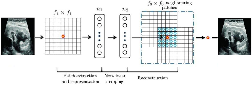

Close

Fig. 1

FSRCNN network structure.

Export to PPT

Feature extraction and representation. The first layer of convolution operation is equivalent to convolving the image, and each convolution kernel corresponds to a basis function so that the image block can be represented by a set of bases (Hamid et al., 2016):$$F_1\left(Y\right)=max\left(0,W_1\ast Y+B_1\right)$$

The size of $W_1$ is $c\times f_1\times f_1\times n_1$. $c$ represents the number of channels input to the image, $f_1\times f_1$ represents the size of the convolution kernel, and $n_1$ is the number of convolution kernels. It can be explained that $W_1$ is performed a convolution operation $n_1$ times on the input image, and the convolution kernel size of each convolution is $c\times f_1\times f_1$. The output corresponds to the $n_1$ number of the feature map. $B_1$ is a vector of h dimensions, and each convolution kernel corresponds to an $n_1$. After convolution, this article responds to the results with an activation function.

Nonlinear mapping. In the first layer of convolution operations, $n_1$ the number of convolution kernels is used in this paper, so $n_1$ the number of feature maps can be obtained. In the nonlinear mapping layer, these $n_1$-dimensional feature vectors are mapped to $n_2$-dimensional feature vectors. The second layer convolution operation can be expressed as (Zhang et al., 2015):$$F_2\left(Y\right)=max\left(0,W_2\ast F_1\left(Y\right)+B_2\right)$$

No more nonlinear mapping layers are used in SRCNN. Increasing the nonlinear mapping layer can improve the quality of the reconstructed image, but it increases the complexity of the model, which leads to more time training for the model.

Image reconstruction. The convolution layer convolves the feature vector of the high-resolution image block outputted from the previous layer and outputs the reconstructed image. The third layer convolution operation can be expressed as:$$F\left(Y\right)=W_3\times F_2\left(Y\right)+B_3$$

Among them, the size of $W_3$ is $n_2\times f_3\times f_3\times c$ and $B_3$ is an $c$-dimensional vector.

Although these three operations play different roles, they are all implemented by convolution. Thus, a three-layer CNN network can be obtained. After the network structure is determined, to learn the mapping function $F$ between the low-resolution image block and the high-resolution image block, this paper needs to continuously optimize the parameter $\theta =\left\{W_1,W_2,W_3,B_1,B_2,B_3\right\}$ in the network to reduce the error value between the reconstructed image and the real high-resolution image. In this paper, the mean square error (MSE) is used as the Loss function of network training:$$L\left(\theta \right)=\frac{1}{n}\sum _{i=1}^n{\left|\left|F\left(Y_i;\theta \right)-X_i\right|\right|}^2$$

Among them, n represents the number of training samples. It has been found through research that when the variables in the above structure are set to $f_1=9,f_3=5,n_1=64,n_2=32$, the trained network has a better reconstruction effect on the image. For the three channels of the color image, this paper only considers the brightness channel of the image, so this paper takes $c=1$. Of course, the values of the variables $f$ and $n$ can also be larger, so that the convolution kernel of the feature extraction in the network is larger, which increases the number of parameters in the network and also increases the amount of sample data required for network training. Therefore, research on this aspect can be further carried out.

Based on SRCNN, a fast image super-resolution reconstruction algorithm, Fast Super-Resolution Convolutional Neural Network (FSRCNN) for short, is proposed. The structure of the network is similar to an hourglass shape, as shown in the following Fig. 1.

The first four layers are convolutional layers, and the last layer is the deconvolution layer. For the sake of easy understanding, the convolutional layer is denoted as $Conv\left(f_i,n_i,c_i\right)$ and the deconvolution layer is denoted as $DeConv\left(f_i,n_i,c_i\right)$. The variables $f_i,n_i\text{and}{c}_i$ are the convolution kernel size, the number of convolution kernels, and the number of channels. The specific operations of each layer are described in detail below.

Feature extraction layer. This layer is similar to the first layer in the SRCNN structure.

After the input image is subjected to a convolution operation of a set of filters, each input image block is represented as a high dimensional feature vector. FSRCNN uses the convolution kernel of $f_i=5$ as the first layer of the convolution kernel. The experiment only trains the channel of the image, so the experiment takes$c_1=1$. Therefore, this paper only needs to determine the number $n_1$ of convolution kernels. From another point of view, $n_1$ can be regarded as the dimension of the low-resolution feature map, which is set to the variable $d$. Then, this article can express the first layer as $Conv\left(5,d_i,1\right)$.

Dimension reduction layer. In SRCNN, the nonlinear mapping layer follows the feature extraction layer, and the high-dimensional low-resolution feature vector is directly mapped to the high-resolution vector space. However, the dimensions of low-resolution feature vectors are generally very high, so the computational complexity of nonlinear mapping layers is usually very high. FSRCNN adds a dimension reduction layer after the feature extraction layer to reduce the low-resolution feature vector dimension $d$ and fix the convolution kernel size $f_2=1$. The filter now acts as a linear combination of low-resolution feature vectors. We take the number of dimensions of the convolution kernel as $n_2=s$ (Here, $s$ is much smaller than $d$), then the low-resolution feature vector dimension is reduced from $d$ to $s$, which greatly reduces the number of parameters. $s$ is the second variable. The second layer can be expressed as $Conv\left(1,s_i,d\right)$.

Nonlinear mapping layer. In the SRCNN structure, when the size of the nonlinear mapping layer convolution kernel is set to $5\times 5$, the image reconstruction effect is significantly better than the nonlinear mapping layer network with the convolution kernel size $1\times 1$. However, if the depth of the network is increased, the computational complexity of the nonlinear mapping layer will increase. In order to balance the contradiction between reconstructed image quality and network training complexity, the convolution kernel size of the nonlinear mapping layer is finally taken $3\times 3$. The number of layers of the nonlinear mapping layer $m$ is another variable that directly affects the computational complexity of reconstructed image quality and model training. The non-linear mapping layer can be represented as $m\times Conv\left(3,3,s\right)$.

Expansion layer. The extension layer can be regarded as inverse processing of the dimension reduction layer. In order to be consistent with the dimension reduction layer, the convolution kernel size of the extension layer is also set to $1\times 1$, and the number of convolution kernels remains the same as the number of convolution kernels of the feature extraction layer. The dimension reduction layer is denoted as $Conv\left(1,s,d\right)$, and then the extension layer can be recorded as $Conv\left(1,d,s\right)$.

Deconvolution layer. The last layer is the deconvolution layer, which uses a set of deconvolution filters to amplify the previous feature image to produce the final reconstructed image. For a convolutional layer, if the convolution kernel convolves the image at a pitch of $k$ steps, the output image is $1/k$ times the input image. Conversely, if the position of the input and output is changed by this paper, the output image will be $k$ times the input image. According to this feature, the output image can be enlarged to a fixed multiple by the deconvolution layer. The deconvolution layer can be expressed as$DeConv\left(9,1,d\right)$.

In this paper, we use the random linear correction unit ($PReLU$) instead of the linear correction unit ($ReLU$). The general form of the activation function $PReLU$ is defined herein as:$$f\left(x_i\right)=max\left(x_i,0\right)+a_{i}min\left(0,x_i\right)$$when $ReLU$ is used as the activation function, this article can only retain information with $x$ greater than 0, and other parts of the information are ignored. Therefore, some information cannot be recovered during image reconstruction. $PReLU$ inherits the property of the $ReLU$ function where $x$ is a positive part. At the same time, in the case where $x$ is less than 0, the function can preserve some useful information by retaining the learnable parameter $a_i$, thereby improving the quality of image reconstruction. The combination of the above five parts forms the FSRCNN model, which can be expressed as:$$\begin{array}{c}Conv\left(5,d,1\right)-PReLU-Conv\left(1,s,d\right)-PReLU-m\times Conv\left(3,s,s\right)-PReLU-Conv\left(1,s,d\right)-\\ PReLU-DeConv\left(9,1,d\right)\end{array}$$

There are three variables $\text{d,}\text{s,}\text{m}$ in the whole structure, which represent the low-resolution feature block vector dimension, the number of the dimension reduction layer convolution kernel and the number of layers of the nonlinear mapping layer. The structure improves the speed of network training and also improves the quality of reconstructed images. For the sake of simplicity, this paper describes the fast-convolutional neural network as $\text{FSRCNN(d, s, m)}$. The computational complexity of this structure is: $\text{O{ (25d + sd + 9ms2 + ds + 81d)SLR} = O{ (9ms2 + 2ds + 106d)SLR }}$. This article does not take into account the parameter $a_i$ of $PReLU$. The structure of the whole $\text{FSRCNN}$ is similar to an hourglass and has symmetry. The experimental results prove that the convolutional neural network of this structure is more efficient for image reconstruction.

Liking SRCNN, this paper uses mean squared error (MSE) as the loss function of the entire convolutional neural network. The final expression of this function is as follows:$$\underset{\theta }{min}=\frac{1}{n}\sum _{i=1}^n{∥F\left(Y_S^i;\theta \right)∥}_2^2$$

In the above formula, $Y_S^i$ and $X^i$ respectively represent the low-resolution and high-resolution sub-block images of the i-th layer in the training process. $F\left(Y_S^i,\theta \right)$ indicates the output of the low-resolution image block through the FSRCNN structure, and the $\theta$ parameter indicates the parameters that need to be optimized for the entire convolutional neural network. All parameters are iterated and optimized by the stochastic gradient descent method. In order to determine the values of the three variables d, s, m, we select d = 48, 56, s = 12, 16 and m = 2, 3, 4 to test, so we can generate a network of 12 different parameters. Comparing the reconstruction effects of different networks on the image, it is concluded that the FSRCNN has the best reconstruction effect on the test image when d = 56, s = 12, m = 4.

3 Results and discussion

Case group: Among the 50 patients, 35 were male, and 15 were female, and the age range of the patients was 20–55 years old, with an average age of 36 years. Informed consent was taken from every patient before the start of the study. There were 3 cases of kidney stones, 7 cases of kidney stones complicated with ureteral stones, 13 cases of ureteral stones, 9 cases of ureteral stenosis, 8 cases of congenital stenosis of renal pelvic ureteral transition, 2 cases of renal pelvic cancer, 1 case of rectal cancer and lower ureteral invasion. Inclusion criteria for cases: (1) B-ultrasound confirmed the patient's unilateral renal mild or moderate hydronephrosis (assembly system expansion less than 3.5 cm). (2) IVP examination of the hydronephrosis showed that it was developed or not developed and the contralateral kidney was normal. (3) The patient's serum creatinine and urea nitrogen are normal. (4) The patient has no history of diabetes, gout, hypertension, urinary tuberculosis or infection. (5) The patient has no renal cyst with a maximum diameter greater than 1.0 cm; (6) The patient had no contraindications for MRI.

Normal control group: 20 healthy volunteers were selected, including 12 males and 8 females, with an age range of 20–54 years and an average age of 35.4 years. It basically matches the age and gender of the case group. The MRI of the kidney of the selected person was not found abnormally, and there was no previous kidney disease, diabetes, hypertension and other related diseases.

IVP inspection method: According to the routine preparation of IVP examination, we first ingested the supine abdomen plain film of the selected person, and injected lopamiro injection (lopamiro, 370 mg I/ml) 40 ml into the selected person (produced by Shanghai Bolai Kexinyi Pharmaceutical Co., Ltd.). At the same time, the Compression belt was applied to the lower abdomen of the selected person, and the filling of the renal pelvis and renal pelvis was observed at 7 min, 15 min, and 30 min after the injection. After filling and satisfying, the film is taken after the loose abdominal pressure belt, and if necessary, the film is delayed, and the longest delay time is 1 h. All patients were strictly followed by the IVP examination procedure and were performed independently by the same doctor.

According to the results of the IVP examination, it was divided into a normal development group, a poor development group, and a non-development group. People with the simultaneous development of kidney pelvis and renal pelvis on the stagnant side and the normal side at 7 min and 15 min of hydronephrosis and with the same density were included in the normal development group of IVP. For those with hydronephrotic kidneys that were delayed and lighter than normal renal pelvis and renal pelvis at 7 min, 15 min and 30 min, they were included in the IVP poorly developed group. The person whose hydronephrosis kidney was still not developed at 1 h was included in the IVP non-developing group. The IVP non-developing group was confirmed by ultrasound, CT, MRU or surgery to have a clear cause of upper urinary tract obstruction. In the absence of the patient's clinical data such as symptoms, signs, and past medical history, the results of the grouping were determined by the two attending physicians.

The ADC, FA image is automatically generated by the FiberTrak software package. The ADC and FA grayscale maps are selected for display. Taking the B = O DTI image as a reference, the corresponding region of interest (ROI) is selected in the ADC and FA grayscale maps of the central layer of the bilateral kidneys. Moreover, the unilateral kidney upper pole, the renal hilum and the lower pole respectively selected 6 circular ROIs in the renal cortex and medulla. The ROI of the renal cortex is within a range of about 3 mm from the surface of the kidney. The ROI of the medulla is taken from the surface of the kidney by less than 3 mm, and blood vessels, artefacts, and renal pelvis are avoided as much as possible (Fig. 1a, b). Each ROI area is between 10 and 20 voxels (Voxel) and is measured repeatedly as described above. In the case group, the unilateral renal cortical or medullary FA value and ADC value were the average value obtained by measuring 6 ROIs of the upper pole, the renal pelvis and the lower pole twice. In the normal control group, the FA value and ADC value of the renal cortex or medulla were the averages of 12 ROIs obtained from the kidneys measuring the upper, middle and lower poles of the kidney.

The medullary tubule structure was imaged at the central level of bilateral kidneys using diffusion tensor tracing imaging (DTT). The FiberTrak software package loads the b = 0 DTI image as an anatomical reference, adjusts the b = 0 DTI image threshold to clearly show the cortical medullary boundary, and browses the image to select the central plane of the double kidney coronal plane. The free curve method then outlines the medullary region (including the renal column) between the cortex and the renal sinus as a seed ROI with a minimum FA of 0.15, a maximum angular change of 27°, and a minimum length of 10 mm. Finally, the software automatically generates a tubule structure map of the medulla region.

The type of image to be reconstructed is a medical ultrasound image (carotid artery ultrasound image). However, the 91-images training set contains images that are type images such as landscapes. Therefore, FSRCNN can only learn related types of image features through training and has no specific features for the reconstruction of medical ultrasound images. Therefore, this experiment additionally selects the common carotid artery map corresponding to the type of image to be reconstructed to train the FSRCNN and compares it with the network obtained by the standard library training to study the reconstruction effect of the training set image type on the ultrasound image.

Fig. 2(a) shows the image of hydronephrosis, in which the hydronephrosis cannot be effectively observed, and there is a certain misdiagnosis in the actual judging process. Based on this, the picture needs to be processed and combined with the CNN neural network of the study for auxiliary diagnosis. In the actual research, the image is sharpened first, and the obtained result is shown in Fig. 3.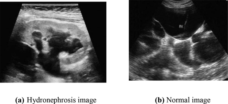

Close

Fig. 2

Comparison of hydronephrosis images and normal images.

Export to PPT

Close

Fig. 3

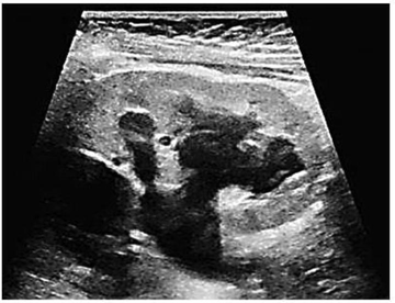
Results after image sharpening.

Export to PPT

As shown in Fig. 3, after the image is sharpened, the sharpness of the image is further improved, and various factors in the image can be clearly displayed. In order to further interpret the image, the image needs to be further processed. In combination with image recognition requirements, the image background needs to be separated, so image grayscale processing is required in the research. The result of grayscale processing is shown in Fig. 4.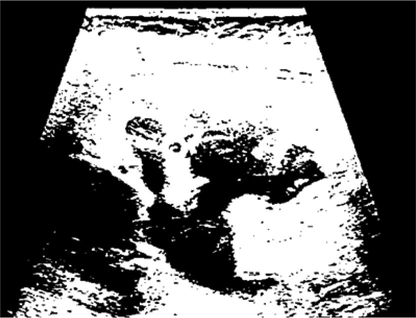

Close

Fig. 4

Image after grayscale processing.

Export to PPT

Through gradation processing, the color interference of the image has been directly eliminated, and the single factor information can be obtained from the image at this time. After that, the image needs to be further processed to further highlight the hydronephrosis factor, and the final test result is obtained. The results of the final treatment are shown in Fig. 5.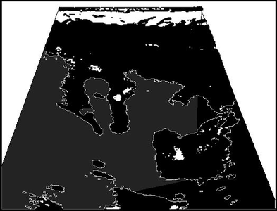

Close

Fig. 5

Image of the test result.

Export to PPT

As shown in Fig. 5, the water accumulation area in the image can be effectively recognized, but there is a certain difference based on the color of the above area, which can be effectively distinguished only by the dividing line. In order to improve the visual effect, the water area is marked with color, and the result is as shown in Fig. 6.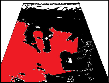

Close

Fig. 6

Results image after color marking.

Export to PPT

As shown in Fig. 6, the color mark in the image is already very clear, and the distribution results of different regions can be clearly observed from the image, thereby effectively improving the diagnosis result. Through the above analysis, it can be seen that the results of this study can obtain effective diagnosis results, that is, the diagnosis results of this study can provide an effective reference for the auxiliary diagnosis of hydronephrosis, which has certain clinical significance.

It is a three-dimensional random diffusion motion, which has not only amplitude but also directionality. Different tissue structures in the human anatomical region may cause differences in the diffusion of water molecules in all directions (Le ihan et al., 2001). If diffusion can occur in all spatial directions, this non-limiting diffusion is called isotropic diffusion. If diffusion can be restricted in one direction by a structure (such as nerve fibers), and the restricted diffusion in all directions is asymmetrical, which is expressed by different intensities in different diffusion directions, it is called anisotropic diffusion (Lu et al., 2006).

In order to explore the effect of the convolution kernel size of the first layer of feature extraction layer on the reconstruction of ultrasound images, based on the initial value of 5 * 5, 7 * 7 and 3 * 3 were used to carry out two experiments. Moreover, this paper uses the two groups of experimental training to perform super-resolution reconstruction of the test images and compares them with the reconstruction effect of the initial value of 5 * 5 network. The network basis of this experiment is US-FSRCNN2 when the number of feature extraction layer convolution kernels is 56. In addition, in the case of ensuring that other parameters are unchanged, only the pretext file describing the network structure is modified. It can be seen from the above results that the CNN neural network method is superior to the traditional recognition algorithm in reconstructing ultrasound images, which shows that the reconstruction method based on the convolutional neural network has certain effectiveness. At the same time, the method of this paper is better than the traditional method in reconstructing ultrasound images. This verifies that in the actual application scenario, the algorithm is also effective for the reconstruction of ultrasound images randomly acquired from the ultrasound imager (Shen and Ebbini, 1996).

In this paper, the thickness of the middle layer of the intima can be accurately obtained, and the thickening of the intima can be found in time to prevent the arteriosclerosis condition in advance. Currently, this indicator has been officially included in the target organ damage category of cardiovascular risk. When observing the reconstructed image of the ultrasound image, the paper can also clearly judge whether the surface of each film is smooth, whether there is crack, and whether plaque is present. If plaque occurs, the doctor needs to judge the type of plaque based on his professional knowledge. The presence of plaque in the arteries is a relatively common problem at present (Glagov, 1994). Over time, some types of plaques will grow up to block the local carotid arteries, and some will fall off into emboli in the bloodstream, which can block the cerebral arteries and cause blood clots (Glagov, 1994). Therefore, the judgment of plaque in the carotid artery is very important. In this paper, the reconstruction result is magnified by 30%. Compared with other algorithms from the visual angle, the algorithm is still relatively clear in the thickness of the film and the plaque (Chan, 2012).

4 Conclusion

In order to improve the clinical effect of an ultrasound-assisted diagnosis of hydronephrosis, this study is aimed at the traditional auxiliary cutting method and proposes an auxiliary diagnosis method based on CNN neural network for the disadvantages of traditional methods. In order to improve the quality of reconstruction and improve the training time of the model, based on SRCNN, a fast image super-resolution reconstruction algorithm is proposed. At the same time, this study combined with CNN neural network for image recognition processing, starting from several angles such as segmentation, grayscale and sharpening. Moreover, the corresponding experiment was designed to analyze, and the clinical effect of the algorithm was analyzed by establishing a control experiment. In addition, in this study, diffusion tensor tracing imaging (DTT) was used to image the medullary tubule structure at the central level of bilateral kidneys. The analysis of results show that the study can obtain effective diagnosis results, that is, the diagnosis results of this study can provide an effective reference for the diagnosis of hydrocephalus ultrasound images, which has certain clinical significance.

References

- Driver head pose estimation using efficient descriptor fusion. EURASIP J. Image Video Process.. 2016;2016(1):2.
- [Google Scholar]
- Hybrid affective computing—keyboard, mouse and touch screen: from review to experiment. Neural Comput. Appl.. 2015;26(6):1277-1296.
- Oriented relative fuzzy connectedness: theory, algorithms, and its applications in hybrid image segmentation methods. EURASIP J. Image Video Process.. 2015;2015(1):1-15.
- Discriminative expression of CD39 and CD73 in cerebrospinal fluid of patients with multiple sclerosis and neuro-Behçet’s disease. Cytokine. 2020;130:155054
- A review of artificial neural networks applications in microwave computer-aided design (invited article) Int. J. RF Microwave Comput. Aided Eng.. 1999;9(3):158-174.
- Cardiovascular Magnetic Resonance of the Arterial Wall in Early Atherosclerosis. 2012.
- Neural networks for computing best rank-one approximations of tensors and its applications. Neurocomputing. 2017;267:114-133.
- Standard plane localization in fetal ultrasound via domain transferred deep neural networks. IEEE J. Biomed. Health. Inf.. 2015;19(5):1627-1636.
- Analysis of solutions for a cerebrospinal fluid model. Nonlinear Anal.: Real World Appl.. 2018;44:417-448.
- Intimal hyperplasia, vascular modeling, and the restenosis problem. Circulation. 1994;89(6):2888-2891.
- Feature exploration for biometric recognition using millimetre wave body images. EURASIP J. Image Video Process.. 2015;2015(1):30.
- Comparative pharmacokinetics of tedizolid in rat plasma and cerebrospinal fluid. Regul. Toxicol. Pharm.. 2019;107:104420
- Delay and link utilization aware routing protocol for wireless multimedia sensor networks. Multimedia Tools Appl.. 2016;75(14):8195-8216.
- MO‐DE‐207B‐06: computer‐aided diagnosis of breast ultrasound images using transfer learning from deep convolutional neural networks. Med. Phys.. 2016;43(6 Part 30) 3705–3705
- Simplified spiking neural network architecture and STDP learning algorithm applied to image classification. EURASIP J. Image Video Process.. 2015;2015(1):4.
- Determination of ceftriaxone concentration in human cerebrospinal fluid by high-performance liquid chromatography with UV detection. J. Chromatogr. B. 2019;1124:161-164.
- Diffusion tensor imaging: concepts and applications. J. Magn. Reson. Imaging. 2001;13(4):534-546.
- Learning to diagnose cirrhosis with liver capsule guided ultrasound image classification. Sensors. 2017;17(1):149.
- Multimedia tool suite for the visualization of drama heritage metadata. Multimedia Tools Appl.. 2016;75(7):3901-3932.
- Three-dimensional characterization of non-gaussian water diffusion in humans using diffusion kurtosis imaging. NMR Biomed.. 2006;19(2):236-247.
- Ultrasound image-based thyroid nodule automatic segmentation using convolutional neural networks. Int. J. Comput. Assist. Radiol. Surg.. 2017;12(11):1895-1910.
- Temporal changes in the cerebrospinal fluid allopregnanolone concentration and hypothalamic-pituitary-adrenal axis activity in sheep during pregnancy and early lactation. Livestock Sci.. 2020;231:103871
- Subarachnoid cerebrospinal fluid is essential for normal development of the cerebral cortex. Semin. Cell Dev. Biol. 2019
- [CrossRef] [Google Scholar]
- Assessment of separation methods for extracellular vesicles from human and mouse brain tissues and human cerebrospinal fluids. Methods. 2020;5:2020.
- Cerebrospinal pharmacokinetic and pharmacodynamic analysis of efficacy of meropenem in paediatric patients with bacterial meningitis. Int. J. Antimicrob. Agents. 2019;54:292-300.
- Sensory neurons contacting the cerebrospinal fluid require the Reissner fiber to detect spinal curvature in vivo. Curr. Biol.. 2020;30 827–839.e4
- Enzyme linked immunosorbent assay for the quantification of nivolumab and pembrolizumab in human serum and cerebrospinal fluid. J. Pharm. Biomed. Anal.. 2019;164:128-134.
- Cerebrospinal fluid and blood lactate concentrations as prognostic biomarkers in dogs with meningoencephalitis of unknown origin. Vet. J.. 2019;254:105395.
- Fighting exclusion: a multimedia mobile app with zombies and maps as a medium for civic engagement and design. Multimedia Tools Appl.. 2017;76(4):4951-4979.
- Towards the design of effective freehand gestural interaction for interactive tv. J. Intell. Fuzzy Syst.. 2016;31(5):2659-2674.
- Diagnostic accuracy of neonatal kidney ultrasound in children having antenatal hydronephrosis without ureter and bladder abnormalities. World J. Urol.. 2015;33(10):1645-1650.
- The effects of both age and sex on irisin levels in paired plasma and cerebrospinal fluid in healthy humans. Peptides. 2019;113:41-51.
- Fuzzy granular classifier approach for spam detection. J. Intell. Fuzzy Syst.. 2017;32(2):1355-1363.
- Cerebrospinal fluid: profiling and fragmentation of gangliosides by ion mobility mass spectrometry. Biochimie. 2020;170:36-48.
- A new coded-excitation ultrasound imaging system. I. Basic principles. IEEE Trans. Ultrason. Ferroelectr. Freq. Control. 1996;43(1):131-140.
- Rapid multiplexed detection of beta-amyloid and total-tau as biomarkers for Alzheimer's disease in cerebrospinal fluid. Nanomed.: Nanotechnol. Biol. Med.. 2018;14:1845-1852.
- Representations of typical hesitant fuzzy rough sets. J. Intell. Fuzzy Syst.. 2016;31(1):457-468.
- A novel approach to rights sharing-enabling digital rights management for mobile multimedia. Multimedia Tools Appl.. 2015;74(16):6255-6271.
- Improved shuffled frog leaping algorithm-based BP neural network and its application in bearing early fault diagnosis. Neural Comput. Appl.. 2016;27(2):375-385.