

Translate this page into:
Trapezoidal breakwater on reducing resonant wave amplitude on a rectangular basin
⁎Corresponding author at: Faculty of Mathematics and Natural Sciences, Institut Teknologi Bandung, Indonesia. ikha.magdalena@itb.ac.id (Ikha Magdalena)
-
Received: ,
Accepted: ,
This article was originally published by Elsevier and was migrated to Scientific Scholar after the change of Publisher.
Abstract
In this study, we delve into the effectiveness of trapezoidal breakwaters in mitigating resonance phenomena. The challenge at hand is to identify the optimal configuration capable of halting resonance. Employing Shallow Water Equations with a friction term to encapsulate the breakwater’s roughness, we analytically solve the model to determine the natural wave period. This period serves as the instigator of an unstoppable harmonic oscillation. Numerically, we use the Finite Volume Method on a Staggered Grid to simulate the model for several cases to pinpoint the infimum value of the natural wave period required to impede resonance phenomena. This research holds significance for those involved in coastal protection design, particularly in the context of trapezoidal breakwaters. The findings contribute to the effective reduction, rather than amplification, of wave height, thereby enhancing the reliability of such coastal protection structures.
Keywords
Trapezoidal breakwater
Resonance phenomena
Optimal configuration
Shallow water equations

1 Introduction
Wave resonance in a certain basin is defined as a linear increase in the amplitude of the natural oscillations occurring in that basin, obtained when a wave enters the basin at a similar frequency as the natural oscillations (Gluskin et al., 2013). The frequency in question is called the natural (resonant) frequency (Rabinovich, 2009). Assuming that the oscillatory system in the said basin is a lossless system, it will absorb more and more energy under resonant excitation, and a steady state is never reached, meaning that the amplitude of the steady state is infinite at resonance (Gluskin et al., 2013). In a real-life situation, the infinite increase of a wave’s amplitude in a certain basin, such as a harbor, port, bay, or coastal area in general, at resonance potentially causes extreme damage in the surrounding area (Farhadzadeh, 2017). This will become more threatening when the wave undergoes resonance and is an extreme wave (e.g., a tsunami) (Yamazaki and Cheung, 2011) or when the general sea level rises due to climate change or monsoons (Dong et al., 2023; Saengsupavanich, 2017; Yun et al., 2023). Therefore, many mitigation efforts have been put in place by installing many types of coastal protection structures (Saengsupavanich, 2022; Saengsupavanich et al., 2023b). For long-term use, many engineers have implemented several approaches to protect coastal areas, such as revetments (Saengsupavanich and Pranzini, 2023), breakwaters (Prukpitikul et al., 2019; Uda, 2022), or beach nourishment (Saengsupavanich et al., 2023a). However, these approaches can be quite expensive and may create a lot of environmental impacts (Pranzini et al., 2015; Sanitwong-Na-Ayutthaya et al., 2023; Saengsupavanich et al., 2022). Hence, a thorough evaluation is required prior to the installation of such a structure, especially to estimate how effective the structure is in reducing the resonant wave’s amplitude.
In the early years, resonances were commonly studied using an experimental approach or field measurement. The studies conducted using experimental approaches date back to the 1990’s, when Martinez and Naverac (1988) carried out experiments, focusing on the effect of the head loss entrance on the resonance. Not too long after, Girolamo (1996) performed experiments to determine the differences in a harbor’s response when a resonance is generated by incident regular free long waves and by incident bound long waves for a narrow and long bay. By conducting field measurements at Marina di Carrara, Italy, Melito et al. (2007) discussed and compared the collected data to numerical predictions using the finite element method. From a mathematical point of view, analytical and numerical models were used to study wave resonance phenomena. For example, analytical and numerical approaches were used to estimate and examine natural frequencies in basins with flat bottoms. Magdalena et al. (2020b) used shallow water equations to investigate the natural frequencies on a said topography in a one-dimensional domain, while Magdalena et al. (2022a) used the same model in a two-dimensional domain. Slightly different, Tsao and Kinnas (2021) applied the New Viscous-Inviscid Interaction (VII) Method to solve the Inviscid-flow problem to address similar issue. In contrast to the three studies mentioned previously, Disimile and Toy (2019) evaluated the behavior of waves with a period that matches the natural frequency of a closed tank by performing small-scale experiments. These studies were then extended to consider basins with a constant slope. Regarding this specific shape of basin, studies done by Wang et al. (2011) and Ezersky et al. (2013) used an analytical approach and/or a previously generated numerical method to investigate resonances, while Magdalena et al. (2021) used both newly developed analytical and numerical approaches to study the phenomena. Further, several researchers started to study resonances on basins with parabolic (Magdalena et al., 2020a), hyperbolic (Wang et al., 2014a), elliptic (Wang et al., 2014b), or exponential (Wang et al., 2015) topography. Other shapes of basins that were not considered regular were also addressed by several researchers, such as Cho and Lee (2000), who examine resonances on a topography with a finite number of steps as well as on a singly-sinusoidally and doubly-sinusoidally varying topography. Niu (2021) also studied a similar issue, but on the area around a circular island instead of the coasts. Other studies, such as the ones done by Cai et al. (2016) and Magdalena et al. (2022b), considered the variations in the basin’s width when discussing the resonance occurrences. In most of the mentioned studies, numerical approaches were also used to simulate wave resonance in the corresponding shapes of basins, evaluate the behavior of the waves under such occurrences, and explore the impacts of certain parameters on resonance. However, these studies only addressed the wave resonance and its behavior under certain conditions, while the solutions to mitigate the damage caused by resonances have not been discussed yet.
In the effort to find a solution to prevent resonance, several studies have been conducted to investigate the effect of a certain type of structure on the reduction of the resonant wave’s amplitude. One of them is the study done by Magdalena et al. (2020b), who discussed the use of an emergent porous medium to mitigate resonance. It was found that the porosity and friction effects of a porous medium play a significant role in reducing the resonant wave’s amplitude. However, the resonance can only be avoided when the porosity and friction factors are fixed at certain values. The same conclusions were reached by Magdalena et al. (2022c, 2023b), Kalashni (2018), who studied the effect of bottom friction on wave resonance. Bottom friction can be a representation of any structure that is submerged and generates a friction effect when it interacts with water but does not alter the topography of the basin, such as coral reefs, rocks, and sediments. Further, studies such as those conducted by Magdalena and Jonathan (2022) and Magdalena et al. (2023a) examined the effect of a coastal hard structure (e.g., breakwater) on wave resonance. The mentioned studies collectively proved that, in addition to providing a friction effect to the system, breakwaters also altered the basin’s topography. Considering that the basin’s topography plays a significant role in the natural frequency at which resonance occurs, installing a breakwater in the basin can potentially prevent wave resonance from occurring. In this case, a correct design is needed, such that the new natural frequency of the basin (which includes breakwaters) will not match the frequency of the typical wave entering the basin. In the case of breakwater’s impact on reducing resonant wave amplitude, Magdalena and Jonathan (2022) and Magdalena et al. (2023a) only addressed rectangular breakwater, which is restricted in terms of the analytically derived natural frequency of the basin.
In this study, we investigate the impact of a trapezoidal breakwater, a more versatile shape compared to the rectangular counterpart, on reducing the amplitude of resonant waves. The challenge in studying the resonance of a trapezoidal breakwater arises from the incorporation of a linear slope function, introducing additional complexity to the problem. Additionally, we assess the correct design of the trapezoidal breakwater to entirely mitigate resonance. The governing equations utilized in this study are the Linear Shallow Water Equations (LSWEs). To achieve our goals, we initially derive the natural frequency of a basin with a trapezoidal breakwater analytically by solving the governing equations. The resulting analytical solution is expressed in the form of Bessel functions. Subsequently, this analytically derived natural frequency is employed to validate the numerical scheme. The numerical scheme developed using the finite volume method on a staggered grid is then utilized to simulate resonance phenomena in a flat-bottomed setting with a trapezoidal breakwater. This simulation allows us to observe the reduction in the amplitude of resonant waves due to the presence of the breakwater.
Furthermore, the validated numerical scheme is employed to explore the breakwater’s potential in preventing resonance. Multiple simulations were conducted with different breakwater designs, resulting in the identification of design(s) capable of eliminating the occurrence of wave resonance.
2 Model and method
The model employed to simulate wave resonance behavior over time is established upon the foundation of the Linear Shallow Water Equations (LSWEs). Subsequently, the governing equations were numerically solved utilizing the Finite Volume Method on a Staggered Grid. Further elaboration on both the governing equations and the numerical scheme is provided in this section.
2.1 Governing equations
To encompass both scenarios, where the breakwater exhibits smooth and rough characteristics, we adapt the LSWEs model proposed by Magdalena and Jonathan (2022), Magdalena et al. (2023a) by introducing a friction factor
within the momentum balance equation (Magdalena et al., 2020a, 2022c, 2023b; Dean and Dalrymple, 1991). The friction coefficient
encapsulates the frictional effects arising from the roughness of the structure. The modified LSWEs are presented as follows in terms of the variables wave elevation
and horizontal velocity
:
Model setup illustration.
2.2 Numerical method
In this section, we outline the discrete formulation of our mathematical model. We employ a staggered finite volume method with an average approach. The grid arrangement discussed herein is visually represented in Fig. 2. The computational domain spans both spatial and temporal domains, designated as and , respectively.
We partition into half and full grids, each with a step’s length of , and discretize into finite time steps of . Eq. (1) is computed on cells centered at , ensuring that the full-grid points exclusively store information related to , , and . Simultaneously, Eq. (2) is calculated on cells centered at , indicating that is stored solely in the half-grid points. This approach facilitates an effective and accurate representation of the system dynamics within the defined computational framework.
Implementing a Leapfrog Scheme, we have formulated the discrete representations of Eqs. (1) and (2). These expressions are articulated as:
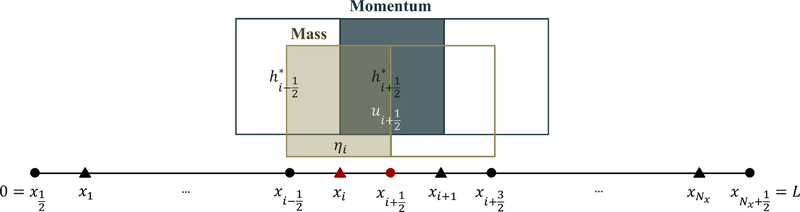
Illustration of finite volume method on a staggered grid.
In these equations, subscripts denote spatial grid points, and superscripts represent time grid points. Additionally, in Eq. (5) is determined implicitly to ensure stability in the numerical scheme. To address Eq. (4), an approximation of on half-grid points, denoted as , is necessary. The notation is estimated using the average value: It is important to highlight that the friction term in Eq. (5) is computed implicitly, a strategic choice made to navigate limitations on numerical stability. Consequently, the stability condition for this scheme remains independent of the friction coefficient, as expressed by:
3 Analytical solution for natural wave period
In this section, we determined the eigenvalue of our mathematical model to obtain the natural period of waves, leading to the occurrence of resonance phenomena. Analogous to the pendulum problem, we unveil the phenomena of unimpeded oscillation and amplify the wave amplitude. Initially, we assume that the initial force applied to our system takes the form of monochromatic waves with a specific frequency of
, such that
By substituting Eqs. (6) and (7) into Eqs. (1) and (2), we obtain the following second-order differential equation:
Subsequently, we utilize Eq. (8) to derive solutions in each domain of
and
, expressed as
, with
in every domain given by:
By performing elimination and applying the following two boundary conditions for the hard wall at
and the minimum condition for
at
, we arrive at:
4 Results
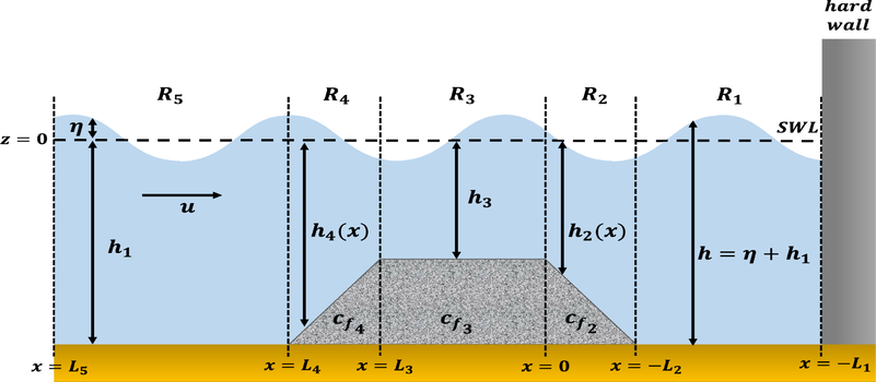
Having formulated the discrete version of our model, we are poised to apply our numerical scheme to explore the manifestation of wave resonance phenomena and to observe whether a trapezoidal breakwater is able to reduce the resonant wave’s amplitude or not. Further, several simulations were performed to find the breakwater’s design that could prevent the resonance from occurring. For all of the computational simulations, the wave is entering from the left-hand side of the spatial domain, and a hard-wall boundary condition ( ) is applied at the right-hand side of the domain. The initial wave entering the basin is defined as , where is the initial amplitude, is the natural frequency of the basin, and is the time variable. The initial condition of the simulations is , representing a calm water condition. Unless stated otherwise, the parameters used in the simulations are the same, which are m, m, , m, s, m, and s. In the next subsections, the analytical formula is used to reproduce the natural frequency of a rectangular (flat bottom) smooth basin, which then compared to the results produced by Magdalena et al. (2020b). Then, the numerical scheme is used to simulate wave resonance in a basin with a trapezoidal breakwater of smooth and rough material. Sensitivity analyses are then conducted to observe the impact of certain parameters on wave resonance. All the numerical simulations are conducted in MATLAB.
4.1 Resonance over a flat bottom
Here, the formulated analytical formula is used to reproduce the natural period in a case where the seafloor is flat and no structure is involved. The resulted natural periods for several scenarios are then compared to the ones generated by Magdalena et al. (2020b) to validate the newly derived formula. The analytical formula for flat bottom that is formulated by Magdalena et al. (2020b) is written as , where is the length of the observed domain. In order to compare both formulas, a few adjustments in the values of , and in Eq. (22) are needed. Table 1 listed two scenarios evaluated in the comparisons between the natural periods produced by Magdalena et al. (2020b) and by Eq. (22). Note that denotes the natural period produced by the formula from Magdalena et al. (2020b) while denotes the ones calculated from Eq. (22). The errors presented in Table 1 were the relative errors calculated using the formula: . It is evident in Table 1 that the errors are all less than 2%, which is considered to be quite small. This outcome shows that the newly derived formula for determining the natural frequencies of a basin with a trapezoidal breakwater may, in fact, be applied to more generic scenarios, such as a flat-bottom basin without a breakwater or with a rectangular breakwater (since the slopes can be adjusted).
(m)
(m)
(s)
(s)
error ()
5
4
5
10
150
5
9.5190
9.5119
0.0750
3
4
5
7
50
7
1.3199
1.3017
1.3789
4.2 Resonance phenomena induced by the trapezoidal breakwater
In this case, we consider a trapezoidal breakwater being placed in a rectangular basin (flat topography). Both the sea floor and the breakwater are considered smooth, which means that the friction effect is neglected or that in the whole domain. The parameters used in these simulations are m, , and s. The frequency of the initial wave used is the natural frequency (natural period) obtained analytically. In this case, the natural frequency is (or s). The other parameters are the same as the ones defined previously. The resulted wave evolution near the wall can be seen in Fig. 3.
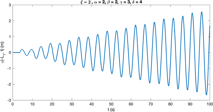
The increase in wave elevation over time, computed after it passes over a smooth trapezoidal breakwater, indicates the occurrence of resonance phenomena.
4.3 The influence of a rough trapezoidal breakwater on resonance wave phenomena
Here, the friction effect is considered present only on the crest of the trapezoidal breakwater (domain ), while the structure’s slopes and the seafloor are still smooth. In each simulation, the parameters related to the breakwater’s configuration are fixed at m, , . The simulations were observed for . The results of the simulations are presented in Fig. 4 with several different values of .
We now see how wave resonance responds to the change in friction coefficient if the friction-affected domain is much bigger. We consider the friction factor to impact the whole trapezoidal breakwater, including its crest and its two slopes (
), while the seafloor is still considered smooth. The parameters are now
m,
,
and
, where the values of
are again varied. The generated wave evolution for each case is shown in Fig. 5.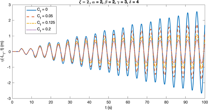
The decrease in the resonant wave’s maximum amplitude, due to the increase in friction coefficient (
) which represents the presence of a trapezoidal breakwater with a rough crest and smooth slopes.
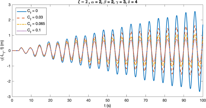
The decrease in the resonant wave’s maximum amplitude, due to the increase in friction coefficient (
) which represents the presence of a trapezoidal breakwater with rough crest and slopes.
4.4 Sensitivity analysis
In this subsection, several parameters are analyzed to observe each parameter’s impact on the wave’s evolution, including the wave’s period and maximum amplitude. Those parameters are which represents the changes in the distance between the breakwater and the wall, which represents the length of the breakwater’s slopes, which represents the changes in the length of the breakwater’s crest, and which represents the changes in the breakwater’s height. For all of the simulations conducted in this subsection, the trapezoidal breakwater is considered rough, which means that the friction factor is considered to exist in subdomains , and , with a fixed friction coefficient .
The first set of simulations to be conducted is the one considering the changes in the breakwater’s distance from the wall ( ). The breakwater’s distance from the wall itself is represented by the term , where the value of is fixed at m and the value of is varied. The other parameters are set to be m, , . Fig. 6 shows how the changes in breakwater’s distance from the wall affect the wave behavior over time.
The next parameter to be discussed is
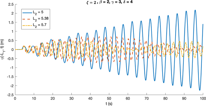
which represents the length of the breakwater’s slope. Therefore, several simulations were done with variations of
. Even though
only represents the length of the front-slope of the breakwater in the setup, in the computation, it also rules the breakwater’s back-slope. Hence, changing
will change both slopes simultaneously. As usual, we set the parameters to be
m,
,
. The value of
is also varied following
to make the distance between the wall and the breakwater fix at
m. The results of the simulations for several values of
are presented in Fig. 7.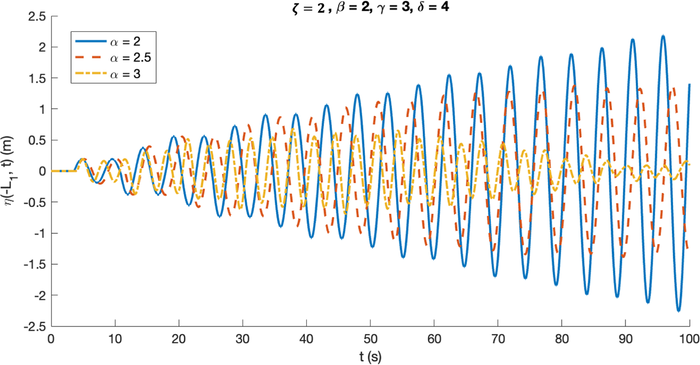
The decrease in the resonant wave’s maximum amplitude, following the increase in the values of
which represents the trapezoidal breakwater’s distance from the wall.
The decrease in the resonant wave’s maximum amplitude, following the increase in the values of
which represents the length of the trapezoidal breakwater’s slopes.
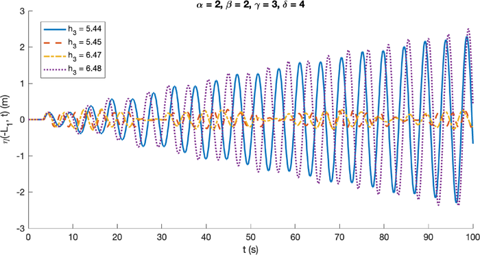
Now, we are examining the effect of another parameter, which is the length of the breakwater’s crest, on the wave maximum amplitude and wave period. This characteristic is represented by . For fixed breakwater’s slopes, varying means varying as well. In this case, we set . However, for a fixed length of the observation domain, the variation of is limited to be less than , while is required. Other than that, m, , are still used. The computational results are shown in Fig. 8.
The last parameter to be examined is the breakwater’s height, represented by the water depth on the crest (
). In this case, the maximum water depth is fixed at
m, such that the parameter
also varies following
. The rest of the parameters are the same, which are
. Fig. 9 shows the simulation results of several breakwater’s heights.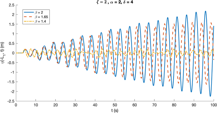
The decrease in the resonant wave’s maximum amplitude, following the increase in the values of
which represents the length of the trapezoidal breakwater’s crest.
The decrease in the resonant wave’s maximum amplitude, following the increase in the values of
which represents the water depth on the trapezoidal breakwater’s crest.
5 Discussion
In Fig. 3, it is evident that the surface elevation near the wall progressively increases throughout the observation time, meeting the criteria for wave resonance phenomena as defined by Gluskin et al. (2013). This indicates that despite the presence of a trapezoidal breakwater in the basin, wave resonance may still occur for a specific set of parameters, particularly if both the seafloor and the breakwater exhibit smooth characteristics. In the subsequent subsections, we delve into the conditions that are essential for preventing resonance, considering factors such as breakwater’s design, position, friction coefficient, and bottom friction.
5.1 Resonant wave’s response to different cases of breakwater’s roughness
The cases depicted in Fig. 4 include friction coefficients of , 0.05, 0.125, and 0.2. These values were selected to illustrate how changes in the friction coefficient impact the evolution of resonant waves and which value can effectively halt resonance. Upon closer examination of Fig. 4, it was observed that despite the consistent increase in the value of in the last three cases (where increases by 0.075), each case had a distinct effect on the maximum amplitude of the resonant wave.
In particular, the third case ( ) demonstrated a reduction of approximately 37% in the maximum amplitude compared to the second case ( ). Conversely, the fourth case ( ) achieved a reduction of only about 31% from the third case. These findings indicate that as increases, its impact on diminishing the maximum amplitude of the resonant wave becomes less significant. Nonetheless, this parameter remains influential in significantly reducing the maximum resonant wave amplitude, with an average reduction of approximately 4.9% for every increase of 0.01 in .
The second piece of information that can be obtained from Fig. 4 is the value of that can stop resonance. A certain set of parameters is considered to be able to stop the resonance if the generated wave amplitude is not increasing infinitely, which means that the last amplitude remains the same or decreases from the previous one. These resonance-stopping parameters were found through a trial-and-error approach. In this case, the resonance is stopped when , which can be seen in Fig. 4 by looking in more detail at the last two amplitudes, which have similar values. This characteristic could not be found in cases where or , since the amplitude keeps on increasing, even with different growth rates. At , the generated wave even seems like a standing wave, where the amplitude is maintained the same throughout the observation time, which means that the resonance barely exists. This result is confirmed by Magdalena et al. (2022c) who stated that at certain values of friction coefficient, a wave resonance is possible to prevent. However, the friction coefficient that is able to prevent resonance in this study is much bigger than the ones generated in Magdalena et al. (2022c) due to the difference in the portion of the water body affected by the friction factor. This difference also impacted the generated natural periods, which are similar for all values of ( ), compared to the ones addressed by Magdalena et al. (2022c), which are varied each time the friction coefficient is changed, since Magdalena et al. (2022c) considered friction factor on the whole observed domain, not just a certain subdomain.
We observed similar results from Fig. 5, where an increase in generates a decrease in the wave’s maximum amplitude. In this case, the values of friction coefficients are . It was found from the simulations that the average reduction generated by an increase of by 0.01 is about 10.2%. This value is larger than the previous case, which makes sense as the portion of the basin’s domain affected by the friction factor was larger in this case compared to the previous one. This means that in this case, the change in affects the wave’s maximum amplitude more significantly than it did in the previous case. Another difference is that in this case, the resonance is able to be stopped at , which is almost two times smaller than the previous case. This is again due to the portion of the basin’s domain affected by the friction factor, which was larger in this case. However, the findings regarding wave period are also applied in this case, where the changes in the friction coefficient barely affect the generated wave period since in all cases.
5.2 Resonant wave’s response to different configurations of trapezoidal breakwater
In Fig. 6, the cases are presented with values of being , with resonance being halted at . This value was determined through a trial-and-error method. Although not clearly depicted in the figure, the wave for exhibited constant oscillations, evidenced by the similarity in its last few amplitudes. A more distinct comparison can be made with the case where , where the wave amplitude infinitely increases. Furthermore, Fig. 6 provides insights into how the breakwater’s location influences the resonant wave’s maximum amplitude and period. It is evident that as the value of increases (indicating a farther breakwater location from the wall), the wave’s maximum amplitude decreases. An increase of by 0.5 (shifting the breakwater 2.5 m further into the ocean from the original position) resulted in a reduction of approximately 43.95% in the maximum amplitude. In other words, each 1 m movement of the breakwater towards the ocean led to a reduction of about 17.58% in the maximum amplitude. However, this finding does not extend to the wave period, as simulations showed fluctuations for different values. The wave periods for were found to be , and 3.2401 s, respectively.
Through a trial-and-error method with various values, three were chosen to represent the effect of changes in the breakwater’s slope: , and 5.7. The case of signifies wave resonance with an infinitely increasing amplitude. When , resonance is completely stopped, evident by the reduction in wave amplitude after approximately s. Unlike previous cases, the transition from resonance to non-resonance in this scenario is abrupt when increases by 0.01 from the resonance state (with resonance still present at ). Furthermore, for (including ), the wave is entirely free from resonance. The wave reduction rate due to the change in showed that an increase of 0.1 m in resulted in an average reduction of approximately 14.05% in the wave’s maximum amplitude. In practical terms, this implies that a gentler breakwater slope is more effective at reducing resonant wave amplitude and ultimately preventing resonance. Similar to the cases, the resulting wave periods fluctuated for a certain range of , with , and 3.3293 s for , and 5.7, respectively.
Fig. 8 displays resonant wave evolution for three different values of : , and 1.4. The breakwater’s crest length is defined by , meaning a smaller corresponds to a shorter breakwater crest. The simulations revealed that resonance could be stopped by implementing a breakwater with a crest length of 8.25 m ( ). Furthermore, a decrease in by 0.1 from resonance ( ) to non-resonance resulted in an approximately 8.06% reduction in maximum amplitude. Conversely, when , the same decrease in led to a more significant reduction (approximately 34.21%). A decrease in also resulted in a decrease in the wave period, with a more pronounced reduction observed when . The wave periods for , and 1.4 were , and 3.2878 s, respectively.
In these simulations, larger corresponds to a shorter breakwater, and vice versa. The results differ slightly from previous cases in terms of the parameter value at which resonance is stopped. Instead of a minimum (as seen in the cases of friction coefficient, , and ) or maximum (as observed in the case of ) value stopping resonance, there are several ranges of values where resonance does not occur. Fig. 9 illustrates that resonance does not occur when m, even though it still occurs when m. Similar to the case of , the transition from resonance to non-resonance is abrupt. However, in this case, resonance also abruptly reappears when m, with even larger wave amplitudes. This suggests a non-resonance range for of m. However, this is not the sole non-resonance range for the breakwater’s height parameter. Within the observed domain of m, a non-resonance state was also observed when m and m. It is essential to consider the feasibility of constructing the breakwater, as when m, the breakwater would be m to m tall, requiring more material and, consequently, increasing construction costs. On the other hand, the range of m may be deemed suitable for design, as the breakwater would not be excessively tall, although the maximum wave amplitude ( m) is larger than for m ( m). Therefore, constructing the breakwater with a height within the range m is recommended.
6 Conclusion
In conclusion, this study developed a mathematical model based on the shallow water equations to simulate resonant wave generation and evolution in a rectangular basin with a submerged trapezoidal breakwater. The model also accounts for the structure’s roughness. In addition, a numerical scheme was formulated using the finite volume method on a staggered grid to solve the model. The validation process, comparing results with a previous study in the absence of a breakwater, demonstrated excellent agreement with errors below 2%. Two scenarios were considered regarding the breakwater’s roughness: roughness only on the crest and roughness on the entire structure. The latter case significantly reduced the wave maximum amplitude compared to the former, aligning with expectations. Increasing the friction factor by 0.01 resulted in a 4.9% reduction in wave maximum amplitude for the first case and a more substantial 10.2% reduction for the second case, over twice that of the first case. Exploring conditions to halt wave resonance under specific predefined setups revealed critical parameters. To prevent resonance, the breakwater should be positioned at least 2.5 times its slope length away from the wall, with both slopes (front and back) requiring a minimum length of 5.38 m. The maximum length of the breakwater’s crest should be approximately 1.65 times the slope’s length. Considering construction cost, a recommended breakwater height range is , showing the largest reduction rate within the examined height range. In light of these findings, we anticipate that this study will contribute valuable insights to the development of coastal protection structures, particularly in preventing wave resonance.
CRediT authorship contribution statement
Ikha Magdalena: Writing – review & editing, Supervision, Software, Methodology, Funding acquisition, Formal analysis, Conceptualization. Yovan Aurelius Darmawan Phang: Writing – original draft, Visualization, Validation, Methodology, Investigation, Formal analysis. Hany Qoshirotur Rif’atin: Writing – original draft, Visualization, Investigation, Formal analysis. Cherdvong Saengsupavanich: Writing – review & editing, Supervision, Resources, Project administration. Sarinya Sanitwong-Na-Ayutthaya: Supervision, Resources, Project administration.
Acknowledgments
This research was supported by Program R3UP managed by The Institute for Science and Technology Development (LPIT) Institut Teknologi Bandung; and by Program Penelitian, Pengabdian kepada Masyarakat dan Inovasi (PPMI) Institut Teknologi Bandung 2024 .
Declaration of competing interest
The authors declare that they have no known competing financial interests or personal relationships that could have appeared to influence the work reported in this paper.
References
- An analytical approach to determining resonance in semi-closed convergent tidal channels. Coast. Eng.. 2016;58(3) 1650009–1–1650009–37
- [CrossRef] [Google Scholar]
- Resonant reflection of waves over sinusoidally varying topographies. J. Coast. Res.. 2000;16(3):870-876.
- [Google Scholar]
- Advanced Series on Ocean Engineering. Singapore: World Scientific Publ.; 1991. chapter Water wave mechanics for engineer and scientists
- The imaging of fluid sloshing within a closed tank undergoing oscillations. Results Eng.. 2019;2:100014
- [CrossRef] [Google Scholar]
- Adaptation of coastal defence structure as a mechanism to alleviate coastal erosion in monsoon dominated coast of Peninsular Malaysia. J. Environ. Manag.. 2023;333:117391
- [Google Scholar]
- Resonance phenomena at the long wave run-up on the coast. Nat. Hazards Earth Syst. Sci.. 2013;13:2745-2752.
- [CrossRef] [Google Scholar]
- A study of Lake Erie seiche and low frequency water level fluctuations in the presence of surface ice. Ocean Eng.. 2017;135:117-136.
- [CrossRef] [Google Scholar]
- An experiment on harbour resonance induced by incident regular waves and irregular short waves. Coast. Eng.. 1996;27(1–2):47-66.
- [CrossRef] [Google Scholar]
- One more tool for understanding resonance and the way for a new definition. J. Eng.. 2013;2013:414109
- [CrossRef] [Google Scholar]
- Resonant excitation of Baroclinic waves in the presence of Ekman friction. Izv. Atmos. Ocean. Phys.. 2018;54:109-113.
- [CrossRef] [Google Scholar]
- Wave resonance phenomena in 2Dxy rectangular basin. Eng. Lett.. 2022;30(4):1596-1602.
- [Google Scholar]
- Water waves resonance and its interaction with submerged breakwater. Results Eng.. 2022;13:100343
- [CrossRef] [Google Scholar]
- Mathematical model for two-submerged breakwaters on preventing wave resonance. Eng. Lett.. 2023;31(3):45-49.
- [Google Scholar]
- Resonant periods of seiches in semi-closed basins with complex bottom topography. Fluids. 2021;6(5):181.
- [CrossRef] [Google Scholar]
- Derivation of fundamental resonant period in width-varying semi-closed basins using modified SWE. J. King Saud Univ., Eng. Sci.. 2022;34(8):102266
- [CrossRef] [Google Scholar]
- Shallow water equations on modeling resonant waves evolution in a rough varying-width basin. Proc. Inst. Mech. Eng. Part M: J. Eng. Marit. Environ. 2023
- [CrossRef] [Google Scholar]
- Analytical and numerical studies for seiches in a closed basin with bottom friction. Theor. Appl. Mech. Lett.. 2020;10(6):429-437.
- [CrossRef] [Google Scholar]
- Seiches and harbour oscillations in a porous semi-closed basin. Appl. Math. Comput.. 2020;369:124835
- [CrossRef] [Google Scholar]
- An experimental study of harbour resonance phenomena. Coast. Eng. Proc.. 1988;1(21):18.
- [CrossRef] [Google Scholar]
- Field measurements of harbour resonance at marina di carrara. In: Coastal Engineering 2006 - 30th International Conference. 2007.
- [CrossRef] [Google Scholar]
- Resonance of long waves around a circular island and its relation to edge waves. Eur. J. Mech. B Fluids. 2021;86:15-24.
- [CrossRef] [Google Scholar]
- Aspects of coastal erosion and protection in Europe. J. Coast. Conserv.. 2015;19:445-459.
- [CrossRef] [Google Scholar]
- An evaluation of a new offshore breakwater at Sattahip Port, Thailand. Marit. Technol. Res.. 2019;1(1):15-22.
- [Google Scholar]
- Kim Y.C., ed. Chapter 9: Seiches and Harbor Oscillations in Handbook of Coastal and Ocean Engineering. Singapore: World Scientific Publ.; 2009. p. :193-236.
- Elevated water level from wind along the Gulf of Thailand. Thalassas. 2017;33(2):179-185.
- [Google Scholar]
- Successful coastal protection by step concrete revetments in Thailand. IOP Conf. Ser. Earth Environ. Sci.. 2022;1072(1):012002
- [Google Scholar]
- Environmental impact of submerged and emerged breakwaters. Heliyon. 2022;8(12):e12626
- [Google Scholar]
- The 2021-procedure for coastal protection by revetments in Thailand. J. Appl. Water Eng. Res.. 2023;11(2):303-316.
- [Google Scholar]
- Jeopardizing the environment with beach nourishment. Sci. Total Environ.. 2023;868:161485
- [Google Scholar]
- Current challenges in coastal erosion management for southern Asian regions: examples from Thailand, Malaysia, and Sri Lanka. Anthropocene Coasts. 2023;6(1):15.
- [Google Scholar]
- Local simulation of sloshing jet in a rolling tank by viscous-inviscid interaction method. Results Eng.. 2021;11:100270
- [CrossRef] [Google Scholar]
- Fundamental issues in Japan’s coastal management system for the prevention of beach erosion. Marit. Technol. Res.. 2022;4(1):251788
- [Google Scholar]
- An analytic investigation of oscillations within a harbor of constant slope. Ocean Eng.. 2011;38:479-486.
- [CrossRef] [Google Scholar]
- Theoretical analysis of harbor resonance in harbor with an exponential bottom profile. China Ocean Eng.. 2015;29(6):821-834.
- [CrossRef] [Google Scholar]
- Analytical solutions for oscillations in a harbor with a hyperbolic-cosine squared bottom. Ocean Eng.. 2014;83:16-23.
- [CrossRef] [Google Scholar]
- An analytical solution for oscillations within an elliptical harbor. Eng. Mech.. 2014;31(4):252-256.
- [CrossRef] [Google Scholar]
- Shelf resonance and impact of near-field tsunami generated by the 2010 Chile earthquake. Geophys. Res. Lett.. 2011;38(12):L12605.
- [CrossRef] [Google Scholar]
- The morphodynamics of wave on a monsoon-dominated coasts: West coast of GoT. Reg. Stud. Mar. Sci.. 2023;57:102729
- [Google Scholar]


