

Translate this page into:
Total factor energy efficiency in regions of China: An empirical analysis on SBM-DEA model with undesired generation
-
Received: ,
Accepted: ,
This article was originally published by Elsevier and was migrated to Scientific Scholar after the change of Publisher.
Peer review under responsibility of King Saud University.
Abstract
Due to the imbalance of regional development and the different energy efficiency of different regions in China, it is necessary to measure the total factor energy efficiency of various economic zones and get the actual situation of each region. The paper uses SBM-DEA Model considering undesired generations to measure the total factor energy efficiency in different regions of China. When analyzing the situation of multiple inputs and multiple outputs, the paper will adopt a decision making-unit that measures multiple inputs and outputs. Thirty provinces and municipalities are divided into eight economic zones by using the State Council’s division method. The average annual total factor energy measurement value in China from 2005 to 2016 is 0.4559 under the consideration of environmental constraints. With the existing technology and the constant investment scale, there is still a 50% increase in this value. This provides a theoretical upside for the further transformation and upgrading of China’s energy production capacity and the reform of the supply side. Then it uses Moran index to get the spatial correlation of TFEE separately. It shows that there is a significant spatial positive correlation of China’s total factor energy efficiency. The conclusion is that China’s total factor energy efficiency has not increased with economic growth, and the regional gap is large, and there is room for improvement of 50%. It also shows that there is a positive spatial correlation among regional TFEE values. That is, high TFEE value in certain area could promote the value of surrounding provinces, indicating that China’s current economic growth is still dominated by energy consumption, and China is also in the middle and late stages of industrialization.
Keywords
SBM-DEA Model
Total factor energy efficiency
Moran index
Spatial correlation test

1 Introduction
Energy has always placed a prominent position in the economic development of all countries. But what comes with it is the serious waste of resources and the pollution of the ecological environment. In order to embark on a sustainable development path with Chinese characteristics, China must improve energy efficiency and reduce the intensity of energy consumption. In addition, the energy resources are relatively abundant, and per capita energy resources are low (Yu et al., 2018). According to the “China Energy Development Report 2017” released by the General Regulations of the Electricity Regulatory Institute on April 11, 2018, in 2017, China’s total energy consumption reached 4.49 billion tons of standard coal, which is an increase of 2.9% compared with the total energy consumption in 2016, and the growth rate is 1.5 percentage points higher than that of 1.4% in 2016. Among the total consumption of energy, coal accounted for 60.4%, clean energy accounted for 20.8%, compared with last year, coal consumption decreased by 1.6 percentage points and clean energy consumption increased by 1.3 percentage points (Peng et al., 2018). Despite the supply-side reform, the entire energy consumption structure is gradually optimized, but the use of energy is still relatively extensive, and the waste is serious (Liu, 2018). So it is particularly necessary to improve energy efficiency. However, due to the imbalance of regional development and the different energy efficiency of different regions, it is necessary to measure the total factor energy efficiency (TFEE) of various economic zones in China and get the actual situation of each region.
2 Literature review
Some researchers proposed total factor energy efficiency considering of multiple input factors (Hu and Wang, 2006). The indicator makes the measurement of energy efficiency more scientific. Therefore, scholars have explored the energy efficiency of total factors on their basis and achieved more results. On the one hand, it is the measurement of total factor energy efficiency. For example, in other study, they measured the energy efficiency of various provinces and cities in China between 1995 and 2004 through the panel model, and concluded that the energy efficiency gaps of the provinces are large and rise first and then fall (Wei and Shen, 2007). The super-efficiency DEA model with the same scale including the knowledge stock in the production function, and empirically study the energy efficiency of all provinces in China and raise the impact of energy endowment on energy efficiency (Andersen 1993). The combination of DEA and malquist index to calculate the index of the province’s provincial total factor energy efficiency change (Qu, 2009). In other study, researchers have made their own contributions in measuring energy efficiency (Bai and Hui, 2017; Fan et al., 2013).
Another aspect is about considering undesired outputs in TFEE, that is, adding more environmental factors. Some scholars considers environmental pollution and uses the Tobin model to study the influencing factors of energy efficiency. According to the cointegration theory and the ECM model China’s total factor energy efficiency is the Granger cause of economic pollution of environmental pollution (Li et al., 2010) other scholars introduce carbon emission constraints, and discussed the time trends and influencing factors of energy efficiency (Lam et al., 2016). Based on the above studies of the total factor energy efficiency, sulfur dioxide and carbon dioxide are considered simultaneously in the model. In addition, there are few studies on regional energy efficiency regional correlations (Li and Hu, 2012; Lin et al., 2017). Therefore, this paper measures energy efficiency on the basis of environmental factors, and tests the regional correlation of energy efficiency in China, providing empirical evidence for energy efficiency improvement and regional cooperation in various regions (Shi and Shen, 2008).
3 Research methods, models and data
3.1 Research methods and models
3.1.1 Energy efficiency measurement
Data Envelopment Analysis (DEA), a non-parametric technical efficiency analysis method, was first proposed by the American Charners, Cooper and Rhodes in 1978. DEA has a wide range of applications and relatively simple principles (Tinbergen, 1942). Especially when analyzing the situation of multiple inputs and multiple outputs, DEA has unparalleled special advantages. So the paper will adopt a decision making-unit (DMU) that measures multiple inputs and outputs. That is called Non-directional, non-radial SBM—DEA model (Tone, 2001; Olmos et al., 2012). The traditional and basic DEA model includes CCR model (Constant Return Scale, CRS) and BBC model (Variable Return Scale, VRS). Those two models are tools for measuring and evaluating the efficiency of DMU with multiple-input, multiple-output, and the same types.
In the equation (1), θ represents the efficiency value of the jth decision unit, and 0 < θ < 1. When θ 1, it is the optimal solution, indicating that the decision unit () is in a relatively valid state at this time. The BBC model is based on the CCR model to increase the constraint . Both CCR and BBC models take radial and angular measures, Tone (2001) proposed a non-radial, non-angled, slack-based measure (SBM) efficiency assessment model that can improve radial (input–output proportional changes to achieve effective) models that are not considered for input–output slack problem (The DMU has invested too much or the output is too little to cause invalidity). That is, if there is excessive input or insufficient output, using the radial DEA model to measure factor efficiency will result in an overestimation of the efficiency of the DEA model; if there are multiple aspects of the input or output of the evaluation object, the use of the angle DEA model may produce deviations in the efficiency measurement results (Lin and Tan, 2016). Based on formula (1), SBM model adds to indicate the excess amount of input and indicates the deficiency of output, which is the slack variable considered by SBM model. At this time, the efficiency evaluation model of could be expressed as:
Among them, is the input–output value of period t of the production unit, represents the slack vector of the input–output (Patterson, 1996). Tone proved that it is technically effective when the slack amount of the CCR model is zero and the efficiency value is greater than or equal to the SBM efficiency value. With the gradual deepening of the study of TFEE, Tone built an SBM model with undesired outputs in 2003:
Equation (3) is an SBM—DEA model with constant scale returns and contains undesired outputs. are input and output values in period t, is a slack variable of input–output. When these variables are greater than or equal to 0, they indicate excessive use of energy inputs, underproduction of expected outputs, and excessive emissions of undesirable outputs. The objective function is strictly decreasing with respect to the slack variable (Kuosmanen, 2012; Lei, 2010; Li and Cheng, 2008). The value of is in the range of 0 to 1, and it can reach 1, when , the corresponding are 0, indicating that the decision unit is fully effective. When the ρ value is<1, it also shows that there is energy waste in the decision-making unit and the efficiency is lost (Li, 2012; Ma, 2017; O’Donnell et al., 2008). The input or output can be further improved. The difference between formula (3) and the basic formula (1) is that slack variables are added to the objective function. While solving the problems of input and output relaxation, the problems associated with unintended output could also be solved.
3.1.2 Spatial correlation test
Spatial autocorrelation is a spatial statistical method, which is mainly used to verify the interactions among regions. Among them, the global Moran index () is a commonly used spatial autocorrelation method (Honma, 2014). Its calculation formula is as follows:
In the formula = , =, S is the total factor energy efficiency value. Standard deviation, i and j denote the i-th and j-th provinces, represent observations in province i, j. In this paper, they represent the total factor energy efficiency of the provinces respectively. is the (i, j) element of the binary contiguous space weight matrix. When the i-th province shares the common border with the j-th governorate, they are considered to be adjacent and named the number 1, that is = 1; When the i-th region and the j-th region do not have a common boundary, they are considered non-adjacent and assigned the number 0, that is, = 0. The value of Moran^’ I is between (-1, 1), and Moran^’ I > 0 indicates positive spatial correlation among regions, which shows that provinces with higher total factor energy efficiency are adjacent, and provinces with lower total factor energy efficiency are adjacent to provinces with the same situation (Sun, 2002; Wang et al., 2019). Moran^’ I < 0 indicates negative spatial correlation between regions, which shows that provinces with higher total factor energy efficiency are surrounded by provinces with lower ones, or provinces with lower efficiency are surrounded by higher ones (Borozan and Djula, 2018). Moran^’ I = 0 indicates that there is no spatial correlation between regions, which shows that total factor energy efficiency values in provinces have nothing to do with each other.
The significance test of is mainly performed by obeying the standard normal distribution Z statistic. Z is calculated as follows:
In the formula ,
,
=.
3.2 Research data and variable selection
3.2.1 Data sources
This paper uses the panel data of 30 provinces (without Tibet because it lacks energy data) and cities in Mainland China for the period of 2005–2016 (Borozan et al., 2018; Brian and Bengt, 2010). In this process, it learns from the concrete ideas of the eight integrated economic zones of the Development Research Center of the State Council, divides the 30 provinces and cities in the sample, and explores the differences in the energy efficiency between regions and the correlations between provinces in one region (Ceylan and Gunay, 2010). In the measurement of total factor energy efficiency, the data used are all derived from the China Statistical Yearbook of the “China Statistical Yearbook 2005” to the “China Statistical Yearbook 2017” for 12 years, the “2016 China Energy Statistical Yearbook”, and Statistical Yearbook in various provinces and cities during 2005–2017 years, and some other data are supplemented through the website of the National Bureau of Statistics and the websites of provincial and municipal statistics bureaus (Chen and Cheng, 2010).
3.2.2 Variable selection
First, selects the input indicators.
3.2.2.1 Energy
The conversion coefficient of the consumption statistics of coal, coke, crude oil, gasoline, kerosene, diesel, fuel oil, and natural gas from 30 provinces and cities from 2005 to 2016 was selected (Table 1) and converted into standard coal (10,000 tons Standard coal).
Energy type
Index coefficient (kg standard coal/kg)
Carbon emission coefficient (kg CO2/TJ)
Energy type
Index coefficient (kg standard coal/kg)
Carbon emission coefficient (kg CO2/TJ)
Raw Coal
0.7143
94,600
Kerosene
1.4714
71,900
Coke
0.9714
94,600
Diesel
1.4571
74,100
Crude
1.4286
73,300
Fuel oil
1.4286
77,400
Gasoline
1.4714
69,300
Natural Gas
1.3300*10^3
56,100
3.2.2.2 Capital
Scholars usually use capital stock as a proxy variable for capital investment. However, statistics on the stock of investment in fixed assets have not yet been compiled in statistical data in China. And there will be some deviation from the results by using different methods (De et al., 2017; Dong, 2008). Therefore, the paper uses the “perpetual inventory method” to consume the fixed capital stock of various provinces and cities in China. The specific formula is as follows:
is the capital stock of the i-th province in the current year, is the capital stock of the first province in the previous year, δ is the depreciation rate of fixed assets, and is the actual fixed asset investment of the first province in the year (Fleiter et al., 2012). This article refers to Shan Haojie’s (2008) estimation method, taking 10.96% as the depreciation rate, and uses formula (6) to measure the capital stock of the research object. The unit is 100 million yuan.
3.2.2.3 Labor force
In the measurement of the labor force, many foreign documents choose labor time and education as indicators of labor input. However, there is no official statistics on labor time in China (Palmer, 2012; Guo et al., 2006). Therefore the paper selects the number of employees at the end of each year in 30 provinces and cities as the labor input variable, and the unit is 10,000.
3.2.3 Second, selects the output indicators.
3.2.3.1 Expected output
The paper uses GDP as expected output index that can indicate the economic growth. Considering that the capital stock is converted in 2000. In order to ensure the consistency of statistical standards, the GDP deflator of each province announced by the statistical yearbooks was deflated at a constant price of 2000.
3.2.3.2 Undesired factors.
In view of China’s commitment to carbon dioxide emissions under the “Paris Agreement” and waste gas sulfur dioxide is the focus of China’s environmental monitoring, the paper includes the emissions of CO2 and SO2 as non-expected output indicators (Jiang et al., 2018; John et al., 2011). The SO2 data in exhaust emissions is derived from the “China Statistical Yearbook” in the corresponding year and the unit is 10,000 tons.CO2 emissions data have not been covered in the annual statistical yearbook. This paper uses the chemical principle of carbon dioxide production during energy consumption to estimate carbon emissions. The calculation formula is:
is the annual actual consumption of the j-th energy source in the t-th year of a province; is the j-th energy heat value conversion coefficient, which is derived from the average low calorific value of “China Energy Statistical Yearbook”; and are the carbon emission factors for the j-th energy source (see Table 1 below) and carbon oxidation factors, with reference to the Intergovernmental Panel on Climate Change (IPCC) Guidelines for National Greenhouse Gas Emissions Inventory; 44/12 is the molecular weight ratio of carbon dioxide and carbon (Yang et al., 2018). And the CO2 emissions in various provinces and cities during 2005–2016 are estimated.
4 Empirical analyses
4.1 Energy efficiency measurement results
The paper uses the non-radial non-angular SBM-DEA model containing undesired outputs and uses Max-DEApSro6.0 to get the efficiency values in China from 2005 to 2016.
4.1.1 Analysis of time dimension difference characteristics
The time dimension mainly analyzes changes in the total factor energy efficiency from 2005 to 2016 across China. The results are shown in Table 2.
Areas
2005
2006
2007
2008
2009
2010
2011
2012
2013
2014
2015
2016
Average
Beijing
1.0000
1.0000
1.0000
1.0000
1.0000
1.0000
1.0000
1.0000
1.0000
1.0000
1.0000
1.0000
1.0000
Tianjin
0.6691
0.6645
0.6340
0.6442
0.6408
0.6065
0.5974
0.6517
0.6516
0.6349
0.6606
0.7210
0.6480
Hebei
0.3888
0.3876
0.3794
0.3726
0.3632
0.3568
0.3331
0.3377
0.3303
0.3171
0.3173
0.3132
0.3497
Shanxi
0.3150
0.3009
0.2999
0.2869
0.2625
0.2538
0.2410
0.2450
0.2365
0.2193
0.2101
0.2076
0.2566
Inner Mongolia
0.3821
0.3476
0.3312
0.3211
0.3139
0.3057
0.2858
0.2989
0.2839
0.2666
0.2700
0.2724
0.3066
Liaoning
0.5072
0.4899
0.4706
0.4419
0.4422
0.4412
0.4191
0.4307
0.4254
0.3983
0.4020
0.3801
0.4374
Jilin
0.4375
0.4152
0.3925
0.3792
0.3716
0.3577
0.3431
0.3576
0.3489
0.3467
0.3482
0.3499
0.3707
Heilongjiang
0.5208
0.5161
0.4984
0.4941
0.4809
0.4704
0.4510
0.4434
0.4289
0.4130
0.4092
0.3948
0.4601
Shanghai
1.0000
1.0000
1.0000
1.0000
1.0000
1.0000
1.0000
1.0000
1.0000
1.0000
1.0000
1.0000
1.0000
Jiangsu
0.6321
0.6290
0.6237
0.6265
0.6226
0.5934
0.5499
0.5644
0.5546
0.5721
0.5750
0.5629
0.5922
Zhejiang
0.6837
0.6616
0.6388
0.6310
0.6137
0.6132
0.5859
0.6125
0.6115
0.5987
0.6041
0.6050
0.6216
Anhui
0.4141
0.4085
0.3926
0.3770
0.3873
0.3888
0.3738
0.3785
0.3597
0.3580
0.3570
0.3544
0.3791
Fujian
0.8036
0.7810
0.7393
0.7291
0.6332
0.6071
0.5507
0.5690
0.5653
0.5379
0.5431
0.5493
0.6340
Jiangxi
0.4334
0.4195
0.4086
0.4224
0.4453
0.4219
0.3996
0.4109
0.3920
0.4047
0.4015
0.3772
0.4114
Shandong
0.4510
0.4466
0.4424
0.4333
0.4247
0.4113
0.3962
0.3981
0.3981
0.3902
0.3835
0.3687
0.4120
Henan
0.3841
0.3685
0.3527
0.3462
0.3472
0.3290
0.3086
0.3171
0.3048
0.3064
0.3045
0.3064
0.3313
Hubei
0.3862
0.3813
0.3804
0.3974
0.4041
0.3941
0.3746
0.3842
0.3944
0.4000
0.4032
0.4003
0.3917
Hunan
0.4565
0.4596
0.4658
0.4965
0.5287
0.5424
0.5301
0.5464
0.5397
0.5399
0.5286
0.5242
0.5132
Guangdong
1.0000
1.0000
1.0000
1.0000
1.0000
1.0000
1.0000
1.0000
1.0000
1.0000
1.0000
1.0000
1.0000
Guangxi
0.4458
0.4337
0.4136
0.4235
0.4206
0.3698
0.3190
0.3120
0.3088
0.3149
0.3227
0.3129
0.3664
Hainan
1.0000
1.0000
1.0000
0.5058
0.4723
0.4441
0.3960
0.3746
0.3636
0.3407
0.3263
0.3258
0.5458
Chongqing
0.4526
0.4471
0.4514
0.4251
0.4442
0.4497
0.4410
0.4677
0.4950
0.5015
0.5126
0.5224
0.4675
Sichuan
0.4221
0.4160
0.4095
0.3946
0.4102
0.4198
0.4292
0.4421
0.4289
0.4291
0.4403
0.4403
0.4235
Guizhou
0.1996
0.1977
0.2042
0.2126
0.2201
0.2301
0.2375
0.2353
0.2293
0.2184
0.2171
0.2104
0.2177
Yunnan
0.3217
0.3077
0.3006
0.3031
0.3108
0.3024
0.2873
0.2873
0.2811
0.2868
0.2965
0.2905
0.2980
Shanxi
0.3082
0.2943
0.2942
0.2954
0.3036
0.2902
0.2808
0.2815
0.2791
0.2641
0.2664
0.2660
0.2853
Gansu
0.2870
0.2837
0.2768
0.2693
0.2803
0.2793
0.2769
0.2830
0.2778
0.2623
0.2622
0.2625
0.2751
Qinghai
0.2844
0.2668
0.2647
0.2576
0.2602
0.2763
0.2664
0.2586
0.2413
0.2336
0.2390
0.2223
0.2559
Ningxia
0.2061
0.1980
0.1900
0.1855
0.1744
0.1662
0.1536
0.1589
0.1537
0.1426
0.1361
0.1328
0.1665
Xinjiang
0.3274
0.3007
0.2924
0.2904
0.2775
0.2689
0.2533
0.2518
0.2331
0.2133
0.2062
0.1996
0.2596
Average
0.5040
0.4941
0.4849
0.4654
0.4619
0.4530
0.4360
0.4433
0.4372
0.4304
0.4314
0.4291
0.4559
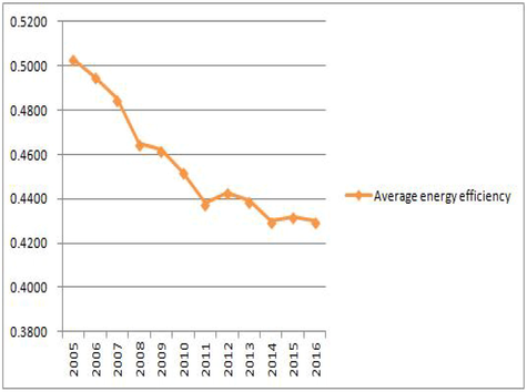
From Table 2, the average annual total factor energy measurement value in China for 12 years is only 0.4559 under the consideration of environmental constraints. With the existing technology and the constant investment scale, there is still a 50% increase in this value (Zhang, 2014). This provides a theoretical upside for the further transformation and upgrading of China’s energy production capacity and the reform of the supply side. Fig. 1 shows the changes of energy efficiency over time in the eight economic zones, and the average value of the national energy efficiency measurement of total factors is transformed into Fig. 2.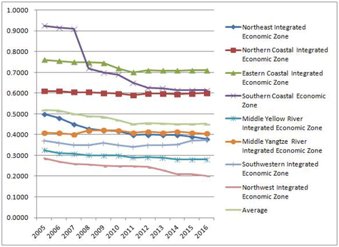
The trend of average energy efficiency of all factors in China from 2005 to 2016.
Trends of total factor energy efficiency values in the eight regions.
In Fig. 1, the overall situation is still consistent with the National Energy Efficiency Trends Chart. The Southern Coastal Economic Zone, Eastern Coastal Economic Zone, and the Northern Coastal Economic Zone are above the mean curve. The integrated economic zone in the middle reaches of the Yangtze River and the Northeast Comprehensive Economic Zone are below the average. Southwest Comprehensive Economic Zone, the Yellow River Integrated Economic Zone, and Northwest Comprehensive Economic Zone are far below the average curve, which shows that the energy efficiency of these areas is even higher. From the curve in the Fig. 2, the southern coastal economic zone of China has experienced a significant decline in 2008, and the overall situation is still at a relatively high level. At the same time, there was a slight increase in 2009 in the Middle Yangtze River Economic Zone and the Southwestern Comprehensive Economic Zone.
At the same time, there was a slight increase in 2009 in the Middle Yangtze River Economic Zone and the Southwestern Comprehensive Economic Zone. According to the data, in 2009, the expected output of these provinces is that the increase in GDP is growing faster than the input, and the undesired output of carbon dioxide and sulfur dioxide emissions is relatively reduced. The Northeast region has been declining from 2005 to 2016. It shows that although there is support for the policy of northeast old industrial bases, the northeast region may not follow the green economic development model very well, and although the trend of economic regression has changed, it also sacrifices local resources and environment.
4.1.2 Analysis of spatial dimension difference characteristics
The spatial dimension mainly discusses the spatial differences in the energy efficiency values of eight regions during 2005–2016 to explore the regional differences under environmental constraints. China has significant differences in geographical conditions, resource endowments and other situations. (Fig. 3).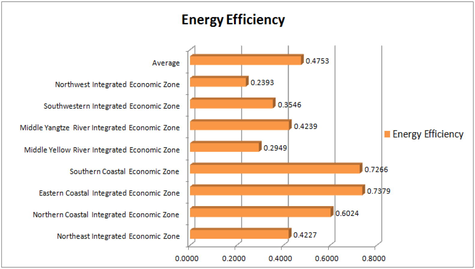
Diagram of total factor energy efficiency in the eight regions.
From Fig. 3, the TFEE of the eastern coastal economic zone and the southern coastal economic zone are relatively high, going 0.7379 and 0.7266 respectively. That is due to the fact that cities in the southeastern coastal areas have developed economies with a relatively high level of openness. At the same time, they have high levels of industrial integration, advanced science and technology, and ample capacity for innovation. The northern coastal integrated economic zone reached 0.6024, mainly because the northern coast includes Beijing, the capital city of China. At the same time there is the coastal city of Tianjin, which has also higher value than the national average of 0.4753. However, the northern coast is not the highest one in the eight regions, mainly because the northern coast also includes Hebei Province and Shandong Province. Although these two provinces have a relatively high level of economic development, they are also accompanied by higher investment and pollution. In particular, Hebei Province has moved into many heavy industrial enterprises in recent years, causing an increase in undesired output. The total factor energy efficiency of the integrated economic zone in the middle reaches of the Yangtze River is 0.4239, which is lower than the national average, followed by the Northeast Comprehensive Economic Zone. It also shows that there are shortages in terms of factors for production such as capital, labor, and technology research and development. The rejuvenation of traditional old industrial bases and measures for the rise of central China are not obvious in the Northeast and the middle and lower reaches of the Yangtze River in the short term or in some important cities. In particular, the Northeast Economic Zone has historical problems in ideology, concepts, and institutional mechanisms have not been solved innovatively, resulting in the failure of improvement in the energy efficiency of all factors. The comprehensive economic zone in the middle Yellow River and the Southwest, Northwest have energy efficiency values below 0.4, and there is room for improvement of 60%. There is still a large gap between the energy efficiency of the region and the southeast coastal areas’. This is related to the original economic system in the west and the transfer of some polluting enterprises. Above all, the spatial changes in energy efficiency values in the eight economic regions of China are: Eastern Coastal Comprehensive Economic Zone Southern Coastal Economic Zone > Northern Coastal Integrated Economic Zone > Middle Yangtze River Integrated Economic Zone > Northeast Integrated Economic Zone > Greater Southwest Comprehensive Economic Zone > Middle Yellow River Integrated Economic Zone > Greater Northwest Comprehensive Economic Zone. It shows a clear spatial aggregate distribution
4.2 Spatial correlation analysis
Using Equation (4) and Equation (5) above, and the Geoda software, the index is shown in Table 3 below:
Year/Indicator
Moran Index
P
Z
SD
2005
0.3588
0.001
3.5606
0.1105
2006
0.3577
0.002
3.5695
0.1108
2007
0.3409
0.003
3.429
0.1104
2008
0.4028
0.001
4.2035
0.1050
2009
0.3830
0.002
4.0188
0.1048
2010
0.3516
0.002
3.7363
0.1242
2011
0.3117
0.004
3.3715
0.1035
2012
0.3357
0.002
3.5704
0.1044
2013
0.3365
0.002
3.5561
0.1050
2014
0.3404
0.002
3.5822
0.1053
2015
0.3433
0.002
3.5987
0.1056
2016
0.3450
0.0020
3.6380
0.1063
Average
0.3656
0.002
3.8135
0.1058
It can be seen from Table 3 that the value of the Morin index I of the total factor energy efficiency from 2005 to 2016 is greater than zero, and the Z value is 1.96, which passed the significance test. It shows that there is a significant spatial positive correlation of China’s total factor energy efficiency.
Fig. 4 reflects the Moran index of all-element energy efficiency in 2008, the highest year for the Moran index, and 2011, the lowest year for the Moran index. Fig. 5 is a scatter plot of the average Moran index for energy efficiency over the 12-year period. In the Moran index scatter chart, the HL region indicates that its own energy efficiency level is higher, and the energy efficiency value of the surrounding regions is lower. The spatial difference between the two is relatively large, that is, there is some heterogeneity in the energy efficiency. However, in Fig. 4 and Fig. 5, there are almost no similar provinces in this scatter plot. The LH region indicates that its own energy efficiency level is relatively low, but the provinces with higher energy efficiency in the neighboring regions are similar to HL in the distribution of provinces with strong spatial heterogeneity. In Fig. 5, although there are some provinces in the LH region, it is also relatively small, indicating that there are fewer provinces with full factor energy efficiency heterogeneity. The HH region is a province with high levels of energy efficiency and relatively high energy efficiency. In the HH area, there are about 8 provinces distributed, indicating an overall higher energy efficiency region in China. In Fig. 4 and Fig. 5, most of the points are located in the LL region, which is the region where the energy efficiency of its own full-element energy efficiency is not high, and the energy efficiency of the full-factor energy of the surrounding regions is not high. In general, there are more HH and LH regions in China’s provinces. It also shows the spatial positive correlation of energy efficiency values of total factors, which shows that space agglomeration is indeed a major feature of China’s total factor energy efficiency. In other words, provinces with higher TFEE are often adjacent to ones with the same situation, and so do the provinces with lower ones. The main reason for this positive correlation in space is that each region learns from each other to achieve the goals of economic growth, improvement of energy structure, energy saving and emission reduction, and reference to new policies, new documents, and new technologies in neighboring regions. So it is possible to use the full positive energy of each region to eliminate the positive correlation of energy efficiency in the provinces and to promote the improvement of energy efficiency of all factors in neighboring provinces.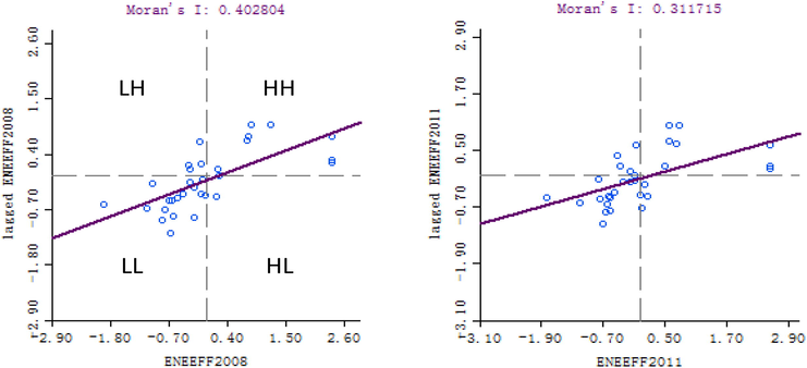
Moran Index I Scatter Diagram of Maximum and Minimum Total Factor Energy Efficiency.
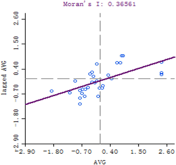
Melanie Moran Index I scatter plot of TFEE.
5 Conclusions and suggestions
Through the above research, the following conclusions are drawn:
5.1 The overall energy efficiency of China has not improved with the improvement of China’s economic development.
In the 12 years from 2005 to 2016, the average energy efficiency of all provinces was only 0.4559, and the energy efficiency level was low. This indicates that China’s overall energy efficiency needs to be improved, energy output is unreasonable, and there is room for improvement of 50%. With the development of China’s economy, China’s total factor energy efficiency still shows an overall downward trend in 2005–2016, indicating that China’s current economic growth is still dominated by energy consumption, and China is also in the middle and late stages of industrialization.
5.2 China’s total factor energy efficiency has large regional differences
China’s TFEE varies widely, including provinces with completely effective production, such as Beijing, Shanghai, and Guangzhou, and provinces with extremely low efficiency, such as Gansu, Ningxia, and Shanxi. The spatial variation of energy efficiency values in China’s eight major economic zones is as follows: Eastern Coastal Comprehensive Economic Zone > South Coastal Economic Zone > Northern Coastal Comprehensive Economic Zone > Middle River Middle Tourist Comprehensive Economic Zone > Northeast Comprehensive Economic Zone > Greater Southwest Comprehensive Economic Zone > Yellow River Midstream Comprehensive Economic Zone > Great Northwest Comprehensive Economic Zone. The spatial aggregation distribution is obvious.
5.3 There is spatial positive correlation in China’s total factor energy efficiency
Through the calculation of Moran index I, it is concluded that there is a positive spatial correlation among provinces. That is, if the total factor energy efficiency of a certain area is high, it can also promote the value of surrounding provinces. Based on the above analysis, it is recommended that the focus should be on improving energy efficiency from the following two aspects:
First, policies to improve energy efficiency should focus on supporting a certain province within a certain region. Through the policy support of the province, the total factor energy efficiency is improved, and then the spillover effect of the total factor energy efficiency is used to achieve the common improvement of the value of the surrounding area. Secondly, eliminating backward production capacity in areas with lower energy efficiency and explore more green development paths. China’s TFEE has a large regional difference. For areas with lower efficiency, the policy should focus on guiding funds to withdraw from overcapacity industries such as steel, nonferrous metals, chemicals, building materials, and thermal power. At the same time, encourage the development of emerging industries such as green environmental protection, high-tech, modern service industries, and encourage the development of green agriculture, green ecology, green tourism, and revitalization of the rural economy in a province suitable for provinces with lower total energy efficiency values. By developing a green economy, it can increase the expected output and improve energy efficiency.
Acknowledgments
The paper is supported by Yue Qi Young Scholar Project (2018QN11), CUMTB and the Fundamental Research Funds for the Central Universities (2009QG09).
Declaration of Competing Interest
The authors declare that they have no known competing financial interests or personal relationships that could have appeared to influence the work reported in this paper.
References
- A procedure for ranking efficient units in data development analysis. Manage. Sci.. 1993;39(10):1261-1264.
- [Google Scholar]
- Is the service industry greener than manufacturing industry? Based on measurement and decomposition of energy productivity. Ind. Eco. Res.. 2017;3:1-14.
- [Google Scholar]
- Technical and total factor energy efficiency of European regions: a two-stage approach. Energy. 2018;152(1):521-532.
- [Google Scholar]
- Analyzing total-factor energy efficiency in Croatian counties: evidence from a non-parametric approach. Central Euro. J. Operat. Res.. 2018;26(3):673-694.
- [Google Scholar]
- Ceylan D., Gunay, E.N.O., 2010. Energy efficiency trends and policies: Cross-country comparison in Europe. International Conference of Economic Modelling. 7(10), Istanbul.
- Endogenous innovation, human development and china’s energy efficiency. China Popul. Res. Environ.. 2010;4:57-62.
- [Google Scholar]
- Application of DEA and statistical inference to model the determinants of biomethane production efficiency: a case study in south China. Appl. Energy. 2017;205:1231-1243.
- [Google Scholar]
- Analysis of the influencing factors of the trend of energy efficiency in China. Indu. Econ. Res.. 2008;1:8-18.
- [Google Scholar]
- Analysis of total factor energy efficiency and potential of the energy-saving and emission – abating in regional of china — based on sbm model of undesired output. Mathemat. Pract. Theory.. 2013;43(7):12-21.
- [Google Scholar]
- Energy efficiency in the German pulp and paper industry-A model-based assessment of saving potentials. Energy.. 2012;40(1):84-99.
- [Google Scholar]
- Does energy efficiency reduce emissions and peak demand? A case study of 50 years of space heating in melbourne. Sustainability.. 2012;4(7):1525-1560.
- [Google Scholar]
- Total-factor energy efficiency of regions in China. Energy Policy. 2006;34:3206-3217.
- [Google Scholar]
- Industry-level total-factor energy efficiency in developed countries: a Japan-centered analysis. Appl. Energy. 2014;119(12):67-78.
- [Google Scholar]
- Total-factor energy efficiency of service industry in China: measurement and influencing factors. J. Beijing Technol. Business Univ. Social Sci.. 2018;33(5):23-32.
- [Google Scholar]
- Energy efficiency and conservation: new legal tools and opportunities. Nat. Resour. Environ.. 2011;25:7-11.
- [Google Scholar]
- Stochastic semi-nonparametric frontier estimation of electricity distribution networks: application of the stoned method in the finish regulatory model. Energy Econ.. 2012;34(6):2189-2199.
- [Google Scholar]
- Progress in waste oil to sustainable energy, with emphasis on pyrolysis techniques. Renew. Sustain. Energy Rev.. 2016;53:741-753.
- [Google Scholar]
- Energy efficiency evaluation and influencing factors of various provinces in China based on DEA method. J. Zhongnan Univ. Econ. Law.. 2010;6:100-108.
- [Google Scholar]
- Relations between total factor energy efficiency and environmental pollution. China Popul. Resour. Environ.. 2010;4:50-56.
- [Google Scholar]
- Ecological total-factor energy efficiency of regions in china. Energy Econ.. 2012;46(3):216-224.
- [Google Scholar]
- Study on the energy efficiency of china and its determinants. Stat. Res.. 2008;10:18-27.
- [Google Scholar]
- Evaluation on regional energy efficiency in china — based on managerial and environmental viewpoints. China Ind Econ.. 2012;6:57-69.
- [Google Scholar]
- Energy efficiency assessment and influencing factors analysis of power system based on new energy industry orientation. Electric Power Const.. 2017;1:123-130.
- [Google Scholar]
- Ecological total-factor energy efficiency of China’s energy intensive industries. Ecol. Ind.. 2016;70:480-497.
- [Google Scholar]
- Economic analysis of methanol production from coal/biomass upgrading. Energy Sour. Part B-Econ. Plan. Policy. 2018;13(1):66-71.
- [Google Scholar]
- The analysis of total factor energy efficiency calculation and influence factors of the three northeast provinces. China Environ. Sci.. 2017;37(2):777-785.
- [Google Scholar]
- Metafrontier frameworks for the study of firm-level efficiencies and technology ratios. Empirical Econ.. 2008;34(2):231-255.
- [Google Scholar]
- On the selection of Finan-cing instruments to push the development of new technologies: appli-cation to clean energy technologies. Energy Policy. 2012;43(6):252-266.
- [Google Scholar]
- What is energy efficiency? concepts, indicators and methodological issues. Energy Policy.. 1996;24(5):377-390.
- [Google Scholar]
- optimization of a hybrid system for solar-wind-based water desalination by reverse osmosis: comparison of approaches. Desalination. 2018;442:16-31.
- [Google Scholar]
- China’s interprovincial total factor energy efficiency change decomposes. J. Quant. Tech. Econ.. 2009;8:29-43.
- [Google Scholar]
- China’s total factor energy efficiency under market segmentation: empirical analysis based on super efficiency DEA method. J. World Econ.. 2008;9:49-59.
- [Google Scholar]
- The decrease in the difference of energy intensities between OECD countries from 1971 to 1998. Energy Policy. 2002;30:631-635.
- [Google Scholar]
- Professor douglas’ production function. revue de linstitut international. De Statistique.. 1942;10(1/2):37-48.
- [Google Scholar]
- A slacks-based measure of efficiency in data envelopment analysis. Eur. J. Oper. Res.. 2001;130(3):498-509.
- [Google Scholar]
- The impact of Internet development on China’s total factor energy efficiency and its network effects. China Popul. Resour. Environ.. 2019;29(1):86-95.
- [Google Scholar]
- Energy efficiency and its influencing factors: an empirical analysis based on DEA. Management World.. 2007;6:66-76.
- [Google Scholar]
- Total factor energy efficiency of the regions along the belt and road: Measurement, decomposition and influence factors analysis. China Environ. Sci.. 2018;38(11):4384-4392.
- [Google Scholar]
- Peak load management based on hybrid power generation and demand response. Energy. 2018;163:969-985.
- [Google Scholar]
- Research on China’s total factor energy efficiency and its influencing factors under carbon emission constraints. Contemp. Finance Econ.. 2014;6:13-22.
- [Google Scholar]


