

Translate this page into:
Time response of fractional automatic control systems
⁎Corresponding author. orfeakos74@gmail.com (A.K. Lazopoulos)
-
Received: ,
Accepted: ,
This article was originally published by Elsevier and was migrated to Scientific Scholar after the change of Publisher.
Peer review under responsibility of King Saud University.
Abstract
*Λ-Fractional Derivative (Λ-FD) is the only non-local Derivative satisfying the demands of Differential Topology. Hence, it is most suitable to investigate the stability of simple SISO and PID control systems. Their behavior is compared in real-time Space in the introduced Λ-Space(Λ-S). According to the definition of Λ-Fractional Derivative and its correspondence to Λ-Space, those Λ-FDs may be viewed as classical Derivatives of transformed new functions and variables in that Space. Firstly the system is analyzed in Λ-S. Afterward, the derived results provide us information about the response of the system in the real Space, by the inverse transformation as proposed from the theory.
Keywords
Λ-Fractional Derivative
Λ-Space
SISO control systems
PID control systems
Stability
Inverse transformation

1 Introduction
Fractional Calculus (FC), originated by Leibnitz, 1849,Liouville, 1832 , and Riemann,1876, is a novel mathematical area applied to modern advances in physics, engineering, etc. Many books describe the applications of FC in these various fields (Kilbas et al., 2006; Samko et al., 1993; Podlubný, 1999a; Oldham and Spanier, 1974). More specifically, as far as engineering is concerned, there are many FC applications in bioengineering, viscoelasticity, electronics, robotics, signal processing, and control theory. Let us point out that fractional Derivatives abolish the local character of the conventional Derivatives. Therefore, they are non-local and most suitable for phenomena that describe the point of interest, as well as the neighborhood around that point. Hence, viscoelasticity and non-local mechanics (Voyiadjis and Sumelka, 2019; Lazopoulos and Lazopoulos, 2019b; Sumelka and Voyiadjis, 2017) along with some aspects of control (Axtell and Bise, 1990, Chen, 2006, Matusu, 2011) and signal processing are favorite fields for FC. Especially in control theory was a new generalization of the classical PID-controller, the idea of P IλDμ-controller (Podlubný, 1999b), involving fractional-order integrator and fractional-order differentiator. That original idea has been proven to be more efficient for the control of fractional-order dynamical systems than the classical one. Incidentally, the contribution of Oustaloup, 1983, 1991, 1994 should be pointed out, successfully introducing the fractional-order controller to develop the so-called CRONE-controller (Commande Robuste d'Ordre Non Entrier controller). That controller also exhibits many advantages, compared to the classical PID-controller. Further applications may be met (Hernández-Acosta et al., 2020; Hernández et al., 2019). Also, ideas concerning short memory phenomena (Podlubný, 1999b), page 203, may be discussed using the non-local fractional Derivatives. Nevertheless, all fractional Derivatives behave like operators, not Derivatives, since they fail to satisfy the demands of Differential Topology for being Derivatives corresponding to differentials. Hence no geometry and consequently, mathematical physics may be established with the use of those fractional Derivatives. In reality, all the well-known fractional Derivatives have mainly an operation character, instead of a derivative's one. However, physicists like to substitute common Derivatives to fractional ones without mathematical justification. There are three prerequisites for defining a derivative corresponding to a differential, Chillingworth, 1976:
Linearity
Leibniz rule
Chain rule
Those perquisites are necessary for defining a differential corresponding to the Derivative. Since no differential geometry, mechanics and physics may be established without mathematically defined Derivative, the use of fractional Derivatives in mathematics and applied sciences, like physics, mechanics, economics, etc. is questionable.
Lazopoulos and Lazopoulos, 2016, trying to fill that gap, proposed the fractional L-derivative. Nevertheless, that effort was not successful, since again the conditions demanded by differential topology were not fully satisfied. Lately, Lazopoulos and Lazopoulos, 2019a; Lazopoulos and Lazopoulos, 2019b proposed the Λ-Fractional Derivative, that is a modification of the fractional L-Derivative, along with the fractional Λ-Space where the Λ-Fractional Derivative behaves according to conventional derivative rules in the Λ-S. Therefore, the main advantage of the method, as mentioned above, is that Λ-Fractional Derivative is a legitimate derivative: It is the only fractional Derivative defined according to the rules demanded by differential geometry. Nevertheless, this advantage requires a price to be paid because it introduces more complexity than the usual methods with fractional operators (i.e., Λ-Space is needed).
In the present article, the stability of simple SISO and PID control systems will be investigated, comparing their behavior in real time–space and Λ-S. It is assumed that the proposed system behavior is governed in Λ-Space from Λ-Fractional Derivatives. According to the previous definition of Λ-FD and its correspondence to Λ-S, those Λ-Fractional Derivatives may be viewed as classical Derivatives of transformed new functions and variables in that Space. The analysis of the system in Λ-Space and the derived results provide us information about the response of the system in the real Space by the inverse transformation according to the proposed theory. Capital letters denote the functions and the variables in Λ-S, and the letter γ indicates the order of the fractional Derivative.
2 The Λ-Fractional Derivative
A very brief outline of fractional calculus will be presented in the present chapter, while the interested reader is referred to refs. (Kilbas et al., 2006; Samko et al., 1993; Podlubný, 1999a) for further study.
The left and right fractional integrals, for a real fractional dimension 0 < γ are defined by,
γ is the order of fractional integrals where Γ(x)=(x-1)! with Γ(γ) Euler’s Gamma function. Further, the left Riemann-Liouville’s fractional derivative (RL) is defined by:
whereas the right Riemann-Liouville's fractional derivative (RL) derivative is defined by:
Let us point out that for the left fractional integrals and Derivative
A similar relation is valid for the right Riemann-Liouville derivative and right fractional integral.
The Λ-Fractional Derivative (Λ-FD) has been defined as
Recalling the definition of the Riemann Liouville's fractional Derivative, Eq. (3), the Λ-FD is expressed by,
Considering as
the Λ-FD appears to behave like a conventional derivative in Λ-S (X, F(X)) with local properties. The Fractional Differential Geometry may be constructed as a conventional differential geometry in Λ-Space, (X, F(X)). Therefore, it is easily understood that the primary goal of this method is to transfer the data from the initial to Λ-S, solve the corresponding differential equation and then go back, through a Riemann-Liouville derivative, to the initial Space, through Eq. (5). The procedure is going to be demonstrated and clarified in the following part of the article.
3 First order systems
Let us consider the following first-order system with feedback in Laplace transformation space:
Where U(s) = R(s) is the input, and Y(s) = C(s) is the output of the system, and T is a time constant that controls the response of the system. The corresponding transfer function of the system can be written as:
We are going to investigate the behavior of such a system in Λ-Space. If we impose a unit step function U(X(t)) in Λ-Space as an input: (See Fig. 1)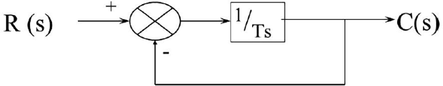
First-order system with feedback.
then the response Y(X(t)) in Λ-Space is given:
Using the relation:
The response Y(X(t)) can be written as:
Declaring: , we take:
To get the response y(t) in real time–space, we use the transformation:
The corresponding input u(t) in real-time Space is: , and its graph for various values of γ is the one below (Fig. 2):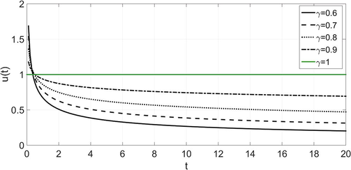
Input u(t) in real time–space, for various values of γ, when the corresponding input U(X(t)) in Λ-Space is a unit step function.
For this input, the corresponding output y(t) in real-time Space (for T = 1) is shown below (Fig. 3):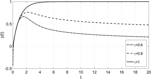
Output y(t) in real time–space, for various values of γ, when the input u(t) is the one shown in Fig. 2.
Let us now consider, the input function of the system in Λ-Space, to be the Dirac delta function or the so-called impulse function U(X) = δ(X(t)). The corresponding output Y(X) of the system is:
Using the relation: , the above equation is written as:
Where
As in previous analysis, the real time–space response y(t) can be found by using the relation:
The input u(t) in the real time–space is:
Using the well-known relation for the Dirac function:
we have for the input:.
For this input, the corresponding output y(t) in real time–space (for T = 1) is shown below (Fig. 4):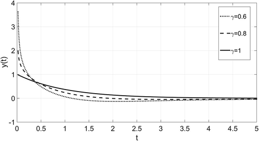
Output y(t) in real time–space, for various values of γ, when the input in Λ-Space is the Dirac Delta Function.
4 Second-Order systems
Let us now investigate the behavior of a standard second-order system, whose transfer function is:
Where ζ is the so-called damping factor of the system.
In the following analysis, a unit step function U(X) is imposed, as an input of the system in Λ-S, and study the system's behavior for values of ζ between 0 and 1. Again, the variable X(t) is the transformed one in Λ-Space of the time variable t in real time–space. It is considered that ωn = 1.
A) Let ζ = 0. Then the output is given as:
The relation can deduce to the time response y(t) in real time–space:
The graph of y(t), for various values of γ, is shown in Fig. 5: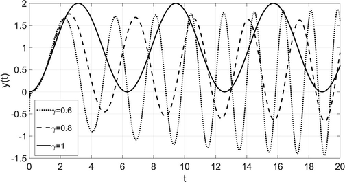
Output y(t) in real time–space, for various values of γ, for ζ = 0 (no damping), and unit step input U(X) in Λ-Space.
B) Let ζ = 1. Then the output is:
Where
The relation can deduce to the time response y(t) in real time–space:
The graph of y(t), for various values of γ, is shown in Fig. 6: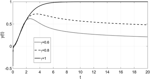
Output y(t) in real time–space, for various values of γ, for ζ = 1 and unit step input U(X) in Λ-Space.
C) Let 0 < ζ < 1. The output in Λ-Space is:
Where
The time response y(t) in real time–space is given by:
The graph of y(t), for ζ = 0.2 and various values of γ, is shown in Fig. 7: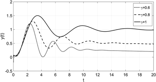
Output y(t) in real time–space, for various values of γ, for ζ = 0.2 and unit step input U(X) in Λ-Space.
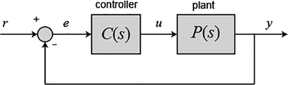
A classical system with a controller.
5 PID controller and the Λ-Fractional Derivative
Let us consider a classical system with a controller as shown below:
In Laplace space R(s) is the input, Y(s) the output, C(s) is the transfer function of the controller, and P(s) is the transfer function of the process. The primary purpose of this design is that the value of the output Y(s) of the system must follow the value of the input (desired value) R(s). The use of the controller C(s) aims to achieve this goal and diminish the error E(s) = R(s)-Y(s).
The transfer function of the construction is:
In our analysis, we'll use a PID controller whose transfer function is:
We'll study a simple 1D physical system that consists of a body of mass M attached to a wall through spring of constant K and a damper of constant b in parallel.
The body can move horizontally when a force F is exerted on it.
Before we continue our analysis, we want to point out that all the values of the system parameters (same in previews systems) are chosen to employ an example and not as corresponding to a particular (experimental) physical system. Our goal is to describe more clearly the behavior of our system.
For M = 1, b = 10, K = 20, the transfer function of such a process is:
Let us investigate the behavior of such a process in Λ-Space. Let T(t) be the transformed variable in Λ-Space of real-time variable t and X(T) the transformed variable in Λ-Space of the x(t) of real time–space. It can be easily proved that without the controller's use, the system's output does not follow the input, and the error is up to 95%.
With the use of the PID controller, the transfer function of the system in Λ-Space becomes:
For ΚD = 50, KP = 350 και KI = 300 and unit step input function F(T):
The output X(T) in Λ-Space is:
It can be shown very quickly that the particular response X(T) in Λ-Space has a short response time and zero error.
By putting T(t) in X(T), we take:
To find x(t) in real time–space, we use:
The input F(t) in real time–space is written as: . The graph of it for various values of γ is shown below:
The corresponding output x(t) for the above inputs F(t) is shown below:
6 The short memory principle
Adapting the idea of short memory in fractional calculus (Podlubný, 1999 a), page 203, of the horizon, introduced in peridynamic deformation theory (Lazopoulos and Lazopoulos, 2019b), the non-local influence is restricted in a neighborhood of time or a point of distance δ. Therefore, the fractional influence is restricted in tε(t-δ, t + δ). If t and f(t) is time and a function of time t, the corresponding configurations in the Λ-Space are defined by,
Let us point out that
Furthermore, the fractional space Λ is defined by lT , Eq.(39) and
Therefore, in the Λ-Space (T, F(T)) the analysis is performed with the conventional local procedure. Furthermore, the results are transferred in the initial Space:
The procedure is repeated for the right Λ-Space, defining the right short memory time variable and right short memory function in the original Space. Indeed, for the right part of the time (t,t + δ) the corresponding Λ-Space is defined by,
Indeed,
Again, the results may be transferred into the initial Space through the relation,
Further details may help to discuss the peridynamic bar problem with the horizon in (Lazopoulos and Lazopoulos, 2019b).
7 Discussion
In the present article, the stability of simple SISO and PID control systems has been studied using non-local mathematically established fractional Derivatives. The well-established non-local Λ-Fractional Derivative, which is transformed in a local one in the Λ-Space, yields a sound and well-established mathematical procedure for creating fractional differential geometry, impossible for other fractional Derivatives that are used with mathematical accuracy in various problems in physics, mechanics, biology, etc. Let us again repeat that no derivation is valid in the initial Space. Derivations are correct only in the Λ-S. Comparison with other fractional Derivatives has been avoided since our perception of mathematics may not be compared to non-mathematically established procedures.
The application of Fractional Calculus in control theory has gained significant attention over a half of century (Castillo-Garcia et al., 2013; Tavazoei, 2014). The study of stability and controllability of such fractional systems is essential because real physical systems seem to obey the logic imposed by FC. Our results and methods (even though they refer to simple systems) aim to contribute to this inquiry, showing that our definition of fractional Derivative may adequately describe the response of real control systems.
8 Conclusions
According to our results from the above analysis, one can conclude for the SISO system the following: For the first-order system, the pole s = −1/T < 0 of G(s) is on the left complex plane, so the system is stable in Λ-Space. It's responses y(t) in real time–space (Figs. 2-4) in both inputs (unit step and impulse) show that it remains stable and in real time–space for values of 0 < γ ≤ 1.
In the case of a second-order system, when the value of ζ is 0 < ζ ≤ 1, the poles are in the left complex plane, and the system is stable for values of 0 < γ ≤ 1 in Λ-Space. It also remains stable in real-time Space (Figs. 6-7). Although in the case of ζ = 0, where the poles s=±jωn are on the imaginary axis, the system is critically stable in Λ-Space. The time response in real time–space (Fig. 5) shows an increase in the amplitude of oscillations, as fractional order γ decreases. It seems that in the case of critical stability in Λ-Space, the system becomes unstable in real time–space.
As far as the PID system is concerned, by comparing Figs. 9 and 10, we can conclude that the output x(t) follows the input F(t) for every value of 0 < γ ≤ 1. So, it seems that the effect of a classical PID controller on a process in Λ-Space continues to have the same impact on the same process, which is governed by Λ-Fractional Derivatives in real time–space.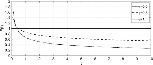
Input F(t) in real time–space, corresponds to a unit step input F(T) in Λ-Space.
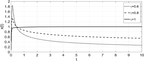
Output x(t) in the real time–space, for various values of γ and unit step input F(T) in Λ-Space.
Finally, by resuming all the above observations, one can deduce that main control behaviors exhibited from classical control systems in Λ-Space, seem to be reproduced in real time–space. However, further investigation on more complicated systems and controllers must be done to establish on a mathematical basis these conclusions.
Declaration of Competing Interest
The authors declare that they have no known competing financial interests or personal relationships that could have appeared to influence the work reported in this paper.
References
- Fractional calculus applications in control systems. In: Proceedings of the 1990 National Aerospace and Electronics Conference. 1990.
- [Google Scholar]
- Castillo-Garcia F. J., San Millan-Rodriguez A., Feliu-Batlle V. and Sanchez-Rodriguez L., 2013, “Fractional-Order PI Control of First-Order Plants with Guaranteed Time Specifications,” J. Appl. Mathemat., 2013.
- Chen Y., 2006. Ubiquitous fractional order controls? In: Proceeding of the 2nd IFAC Workshop on Fractional Differentiation and its Applications, Porto, Portugal.
- Differential topology with a view to applications. London, San Francisco: Pitman; 1976.
- Hernández-Acosta, M. A., Soto-Ruvalcaba, L., Martínez-González, C. L., Trejo-Valdez, M. and Torres-Torres, C., 2019. Optical phase-change in plasmonic monoparticles by a two-wave mixing, Phys. Scr. 94,125802, 9.
- Fractional thermal transport and twisted light induced by an optical two-wave mixing in single-wall carbon nanotubes. Int. J. Thermal Sci.. 2020;147:106136.
- [Google Scholar]
- Theory and Applications of Fractional Differential Equations. Amsterdam: Elsevier; 2006.
- Fractional vector calculus and fractional continuum mechanics. Prog. Fract. Diff. Appl.. 2016;2(1):67-86.
- [Google Scholar]
- On the Mathematical Formulation of Fractional Derivatives. Prog. Fract. Diff. Appl.. 2019;5(4):261-267.
- [Google Scholar]
- Lazopoulos, K. A. & Lazopoulos, A. K., 2019b. On the fractional deformation of a linearly elastic bar, Jnl Mech. Beh. Mat., 28,1–10.
- Leibnitz G.W.,1849. Letter to G. A. L’Hospital, Leibnitzen Mathematishe Schriften, 2, 301-302.
- Sur le calcul des differentielles a indices quelconques. J. Ec. Polytech.. 1832;13:71-162.
- [Google Scholar]
- Application of fractional order calculus in control theory. Int. Jnl. Math. Mod. Meth. App. Sci.. 2011;7(5):1162-1169.
- [Google Scholar]
- The fractional calculus. New York and London: Academic Press; 1974.
- Systèmes Asservis Linéaires d’Ordre Fractionnaire. Paris: Masson; 1983.
- La Commande CRONE. Paris: Hermes; 1991.
- La Robustesse. Paris: Hermes; 1994.
- Fractional Differential Equations (An Introduction to Fractional Derivatives, Fractional Differential Equations, Some Methods of Their Solution and Some of Their Applications). San Diego-Boston-New York-London-Tokyo-Toronto: Academic Press; 1999.
- Fractional-Order Systems and PIλ D μ - Controllers. IEEE Trans. Autom. Control. 1999;44(1):208-214.
- [Google Scholar]
- Riemann B.,1876. Versuch einer allgemeinen Auffassung der Integration and Differentiation. In: Gesammelte Werke, 62.
- Fractional integrals and Derivatives: theory and applications. Amsterdam: Gordon and Breach; 1993.
- Sumelka W., Voyiadjis, G. Z.,2017. A hyperelastic fractional damage material model with memory, Int. Jnl. Sol. & Struct. 124, 151-160.
- Tavazoei M.S., 2014, “Time Response Analysis of Fractional Order Control Systems: A Survey on Recent Results,” Fractional Calculus and Applied Analysis, 17(2).
- Brain modeling in the framework of anisotropic hyperelasticity with time-fractional damage evolution governed by the Caputo-Almeida fractional derivative. J. Mech. Beh. Biom.l Mat.. 2019;89:209-216.
- [Google Scholar]


