Three iterative methods for solving second order nonlinear ODEs arising in physics

M.A. Al-Jawary; M.I. Adwan; G.H. Radhi

doi:10.1016/j.jksus.2018.05.006

View/Download PDF

Buy Reprints

PDF

Translate this page into:

32 (

); 312-323

doi:

10.1016/j.jksus.2018.05.006

Three iterative methods for solving second order nonlinear ODEs arising in physics

M.A. Al-Jawary^⁎, M.I. Adwan, G.H. Radhi

Department of Mathematics, College of Education for Pure Sciences (Ibn AL-Haitham), University of Baghdad, Baghdad, Iraq

⁎Corresponding author. majeed.a.w@ihcoedu.uobaghdad.edu.iq (M.A. Al-Jawary)

Received: 2018-2-16, Accepted: 2018-5-6, Published: 2018-01-01

Disclaimer:
This article was originally published by Elsevier and was migrated to Scientific Scholar after the change of Publisher.

Peer review under responsibility of King Saud University.

Abstract

In this work, three iterative methods have been implemented to solve several second order nonlinear ODEs that arising in physics. The proposed iterative methods are Tamimi-Ansari method (TAM), Daftardar-Jafari method (DJM) and Banach contraction method (BCM). Each method does not require any assumption to deal with nonlinear term. The obtained results are compared numerically with other numerical methods such as the Runge-Kutta 4 (RK4) and Euler methods. In addition, the convergence of the proposed methods is given based on the Banach fixed point theorem. The results of the maximal error remainder values show that the present methods are effective and reliable. The software used for the calculations in this study was Mathematica®10.

Keywords

Iterative methods

Approximate solution

Numerical solution

Runge-Kutta 4 method

Euler method

Show Related Articles from PubMed

1 Introduction

The differential equations have many applications in science and engineering, especially in problems that have the form of nonlinear equations. The applications of nonlinear ordinary differential equations by mathematical scientists and researchers have become more important and interesting. It has been known that these equations describe different types of phenomena such as modeling of dynamics, heat conduction, diffusion, acoustic waves, transport and many others.

The iterative methods are often used to get the approximate solutions for the different nonlinear problems. A new iterative method has been presented in 2011 by Temimi and Ansari (TAM) (Temimi and Ansari, 2011) for solving nonlinear problems. The TAM was inspired from the homotopy analysis method (HAM) (Liao and Chwang, 1998), and used to solve several ODEs (Temimi and Ansari, 2015), PDEs and KdV equations (Ehsani et al., 2013); differential algebraic equations (DAEs) (AL-Jawary and Hatif, 2017); Duffing equations (AL-Jawary and Al-Razaq, 2016); some chemical problems (AL-Jawary and Raham, 2017), thin film flow problem (AL-Jawary, 2017) and Fokker-Planck’s equations (AL-Jawary et al., 2017).

The other proposed method has been proposed in 2006 by Daftardar-Gejji and Jafari, (DJM) (Daftardar-Gejji and Jafari, 2006) to solve nonlinear equations. Also, this method has been used to solve different equations such as fractional differential equations (Daftardar-Gejji and Bhalekar, 2008), partial differential equations (Bhalekar and Daftardar-Gejji, 2008); Volterra integro-differential equations and some applications for the Lane-Emden equations (AL-Jawary and AL-Qaissy, 2015), evolution equations (Bhalekar and Daftardar-Gejji, 2010). This method presented a proper solution which converges to the exact solution “if such solution exists” through successive approximations.

The other iterative method depends on the Banach contraction principle (BCP) (Daftardar-Gejji and Bhalekar, 2009) where it is another iterative method considered as the main source of the metric fixed point theory. The Banach contraction principle also known to be Banach's fixed point theorem (BFPT) has been used to solve various kinds of differential and integral equations (Joshi and Bose, 1985).

In this paper, the TAM, DJM, and BCM will be implemented to solve the nonlinear second order ODEs that arising in physics to get an approximate solutions. These solutions will be compared numerically with another results obtained by the Runge-Kutta and Euler methods to show the validity and the efficiency of the proposed iterative methods. The convergence for these presented methods is also discussed.

This paper is organized as follows: Section 2 reviews the basic ideas of the proposed iterative methods. Section 3 presents the convergence of the proposed methods. Section 4 illustrates the approximate solutions and the numerical simulation for several test problems. Finally, the conclusion has been given in section 5.

2 The basic concepts of three iterative methods

Iterative method is a mathematical procedure generates a sequence of improved approximate solutions for a class of problems. The iterative method leads to the production of an approximate solution which converges to the exact solution when the corresponding sequence is convergent at some given initial approximations.

Let us introduce the following nonlinear differential equation:

(1)

L (y (x)) + N (y (x)) + g (x) = 0,

with the boundary conditions

(2)

B (y, \frac{dy}{dx}) = 0, x \in D

where x represents the independent variable,

y (x)

is the unknown function,

g (x)

is a given known function,

L (\cdot) = \frac{d^{2}}{{dx}^{2}} (\cdot)

is the linear operator,

N (\cdot)

is the nonlinear operator,

B (\cdot)

is a boundary operator. Now, let us begin by introducing the basic ideas of the three iterative methods.

2.1

2.1 The basic idea for the TAM

We first begin by assuming that $y_{0} (x)$ is an initial guess to solve the problem $y (x)$ and the solution begins by solving the following initial value problem (Temimi and Ansari, 2011):

(3)

L (y_{0} (x)) + g (x) = 0, and B (y_{0}, \frac{{dy}_{0}}{dx}) = 0 .

The next approximate solutions are obtained by solving the following problems

(4)

L (y_{1} (x)) + g (x) + N (y_{0} (x)) = 0, and B (y_{1}, \frac{{dy}_{1}}{dx}) = 0 .

and thus we have a simple iterative procedure which is the solution of a set of problems i.e.,

(5)

L (y_{n + 1} (x)) + g (x) + N (y_{n} (x)) = 0, and B (y_{n + 1}, \frac{{dy}_{n + 1}}{dx}) = 0 .

Then, the solution for the problem (1) with (2) is given by

(6)

y = \lim_{n \to \infty} y_{n} .

2.2

2.2 The basic idea for the DJM

Let us apply the inverse operator $L^{- 1} (\cdot) = \int_{0}^{x} \int_{0}^{x} () d τ d τ$ to the nonlinear problem presented by (1) and (2) we have

(7)

y (x) = f (x) + \int_{0}^{x} \int_{0}^{x} N (y (τ)) d τ d τ,

and by reducing the integration from double to single (Wazwaz, 2015); we get the following form

(8)

y (x) = f (x) + \int_{0}^{x} (x - τ) N (y (τ)) d τ,

where f is a known analytic function represents the sum of the available initial conditions and the result of integrating of the function

g

(if such function is available).

The solution $y$ for Eq. (8) can be given by the following series (Daftardar-Gejji and Jafari, 2006):

(9)

y = \sum_{i = 0}^{\infty} y_{i}

Now, the following can be defined

(10)

G_{0} = N (y_{0}),

G_{m} = N (\sum_{i = 0}^{m} y_{i}) - N (\sum_{i = 0}^{m - 1} y_{i}), m ⩾ 1

So, that

N (y)

can decomposed as

N (\sum_{i = 0}^{\infty} y_{i}) = \underset{G_{0}}{\underset{︸}{N (y_{0})}} + \underset{G_{1}}{\underset{︸}{[N (y_{0} + y_{1}) - N (y_{0})]}} + \underset{G_{2}}{\underset{︸}{[N (y_{0} + y_{1} + y_{2}) - N (y_{0} + y_{1})]}} + \underset{G_{3}}{\underset{︸}{[N (y_{0} + y_{1} + y_{2} + y_{3}) - N (y_{0} + y_{1} + y_{2})]}} + \dots .

Moreover, the relation is defined with recurrence so that

(11)

y_{0} = f,

(12)

y_{1} = L (y_{0}) + G_{0},

(13)

y_{m + 1} = L (y_{m}) + G_{m}, m ⩾ 1

Since

L

represents a linear operator

\sum_{i = 0}^{m} L (y_{i}) = L (\sum_{i = 0}^{m} y_{i})

, we may write

\sum_{i = 1}^{m + 1} y_{i} = \sum_{i = 0}^{m} L (y_{i}) + N (\sum_{i = 0}^{m} y_{i}) = L (\sum_{i = 0}^{m} y_{i}) + N (\sum_{i = 0}^{m} y_{i}), m ⩾ 1

So that,

\sum_{i = 0}^{\infty} y_{i} = f + L (\sum_{i = 0}^{\infty} y_{i}) + N (\sum_{i = 0}^{\infty} y_{i})

and the approximate solution will be given in

y_{n} = \sum_{i = 0}^{n} y_{i}, n \in N .

2.3

2.3 The basic idea of the Banach contraction method (BCM)

Consider Eq. (8) as a general functional equation. In order to implement the BCM, we define successive approximations (Daftardar-Gejji and Bhalekar, 2009):

(14)

\begin{matrix} y_{0} = f, \\ y_{1} = y_{0} + N (y_{0}), \\ y_{2} = y_{0} + N (y_{1}), \\ ⋮ \end{matrix}

and so on, we will get successive approximations for

y_{n} (x)

in the following generalized form

(15)

y_{n} = y_{0} + N (y_{n - 1}), n \in N

Therefore, the solution for the relations (14) and (15) will be obtained by

(16)

y = \lim_{n \to \infty} y_{n} .

3 The convergence of the proposed iterative methods

In this section, we present the fundamental theorems and concepts for the convergence (Odibat, 2010) of the presented methods.

The iterations occurred by the DJM are straight used to prove the convergence. However, for the convergence proof of the TAM or BCM, the following procedure should be used for handling Eq. (1) with the given conditions (2). So, we have the terms

(17)

\begin{matrix} v_{0} = y_{0} (x), \\ v_{1} = F [v_{0}], \\ v_{2} = F [v_{0} + v_{1}], \\ ⋮ \\ v_{n + 1} = F [v_{0} + v_{1} + \dots + v_{n}] . \end{matrix}

where F represents the following operator

(18)

F [v_{k}] = S_{k} - \sum_{i = 0}^{k - 1} v_{i} (x), k ⩾ 1 .

In general, the term

S_{k}

is the solution for the problem in the form, for the TAM:

(19)

L (v_{k} (x)) + g (x) + N (\sum_{i = 0}^{k - 1} v_{i} (x)) = 0, k ⩾ 1 .

For the BCM:

(20)

v_{k} = v_{0} + N (\sum_{i = 0}^{k - 1} v_{i} (x)), k ⩾ 1 .

By using the same conditions with the intended iterative technique that will be used. Therefore, we get

y (x) = \lim_{n \to \infty} y_{n} (x) = \sum_{n = 0}^{\infty} v_{n}

. Hence, by using Eqs. (17) and (18), the following solution will be obtained in a series form

(21)

y (x) = \sum_{i = 0}^{\infty} v_{i} (x) .

According to the recursive algorithms of the proposed methods, the sufficient conditions for convergence of these methods can be given in following theorems.

Theorem 4.1

Let F defined in (18), be an operator from a Hilbert space H to H. The series solution $y_{n} (x) = \sum_{i = 0}^{n} v_{i} (x)$ converges if $\exists 0 < γ < 1$ such that $F [v_{0} + v_{1} + \dots + v_{i + 1}] ⩽ γ F [v_{0} + v_{1} + \dots + v_{i}]$ (such that $v_{i + 1} ⩽ γ v_{i}$ ) $\forall i = 0, 1, 2, \dots$ .

This theorem is a special case of Banach’s fixed point theorem which is a sufficient condition to study the convergence.

Proof

See (Odibat, 2010). □

Theorem 4.2

If the series solution $y (x) = \sum_{i = 0}^{\infty} v_{i} (x)$ is convergent, then this series will represent the exact solution of the current nonlinear problem.

Proof

See (Odibat, 2010). □

Theorem 4.3

Suppose that the series solution $\sum_{i = 0}^{\infty} v_{i} (x)$ presented by (21) is convergent to the solution $y (x)$ . If the truncated series $\sum_{i = 0}^{n} v_{i} (x)$ is used as an approximation to the solution of the current problem, then the maximum error $E_{n} (x)$ is estimated by

(22)

E_{n} (x) ⩽ \frac{1}{1 - γ} γ^{n + 1} v_{0} .

Proof

See (Odibat, 2010). □

Theorems 4.1 and 4.2 state that the solutions obtained by one of the presented methods, i.e. the relation (5) (for the TAM), the relation (13) (for the DJM), the relation (15) (for the BCM), or (17), converges to the exact solution under the condition $\exists 0 < ξ < 1$ such that $F [v_{0} + v_{1} + \dots + v_{i + 1}] ⩽ ξ F [v_{0} + v_{1} + \dots + v_{i}]$ (that is $v_{i + 1} ⩽ ξ v_{i}$ ) $\forall i = 0, 1, 2, \dots$ . In another meaning, for each i, if we define the parameters

(23)

β_{i} = \{\begin{matrix} \frac{∥ v_{i + 1} ∥}{∥ v_{i} ∥}, & ∥ v_{i} ∥ \neq 0 \\ 0, & ∥ v_{i} ∥ = 0 \end{matrix}

then the series solution

\sum_{i = 0}^{\infty} v_{i} (x)

for the nonlinear ODE given by (1) will be convergent to the exact solution

y (x)

, when

0 ⩽ β_{i} < 1, \forall i = 0, 1, 2, \dots

. Also, as in Theorem 4.3, the maximum truncation error is estimated to be

y (x) - \sum_{i = 0}^{n} v_{i} ⩽ \frac{1}{1 - β} β^{n + 1} v_{0}

, where

β = \max {β_{i}, i = 0, 1, \dots, n}

4 Test problems

Problem 1:

The Painlevé equation I can be given by the following form (Hesameddini and Peyrovi, 2009)

(24)

y^{″} (x) = 6 y^{2} (x) + x,

with the initial conditions:

y (0) = 0

and

y^{'} (0) = 1

. This problem will be solved by using the three proposed iterative methods.

Solving the problem 1 by the TAM:

In order to solve Eq. (24) by the TAM, we have the following form

(25)

L (y) = y^{″} (x), N (y) = - 6 y (x) and g (x) = - x .

The initial problem will be:

(26)

L (y_{0} (x)) = x, with y_{0} (0) and y_{0}^{'} (0) = 1 .

We can get the next problems from the generalized following relationship

(27)

L (y_{n + 1} (x)) + g (x) + N (y_{n} (x)) = 0, y_{n + 1} (0) = a and y_{n + 1}^{'} (0) = b .

Firstly, to get the zero approximation

y_{0} (x)

, the following initial problem must be solved:

(28)

y_{0}^{″} (x) = x,

By integrating both sides of Eq. (28) twice from 0 to x and substituting the initial conditions

y_{0} (0) = 0

and

y_{0}^{'} (0) = 1

, we get

y_{0} (x) = x + \frac{x^{3}}{6},

In a similar way, the rest of the other iterations can be carried out, the first iteration can be obtained by calculating

(29)

y_{1}^{″} (x) = 6 y_{0}^{2} (x) + x, with y_{1} (0) = 0 and y_{1}^{'} (0) = 1,

Then, the approximate solution for Eq. (29) will be then:

y_{1} (x) = x + \frac{x^{3}}{6} + \frac{x^{4}}{2} + \frac{x^{6}}{15} + \frac{x^{8}}{336} +, \dots

The second iteration

y_{2} (x)

can be obtained from solving the following

(30)

y_{2}^{″} (x) = 6 y_{1}^{2} (x) + x, with y_{2} (0) = 0 and y_{2}^{'} (0) = 1,

Then, by solving Eq. (30), we obtain:

y_{2} (x) = x + \frac{x^{3}}{6} + \frac{x^{4}}{2} + \frac{x^{6}}{15} + \frac{x^{7}}{7} + \frac{x^{8}}{336} + \frac{x^{9}}{40} + \frac{x^{10}}{60} + \frac{71 x^{11}}{46200} + \frac{x^{12}}{330} + \frac{x^{13}}{26208} + \frac{187 x^{14}}{764400} + \frac{x^{16}}{100800} + \frac{x^{18}}{5757696} + \dots

Thus, we continue to obtain the approximations till $n = 5$ for $y_{n} (x)$ , but for brevity the terms are not listed.

Solving the problem 1 by the DJM:

Consider the Eq. (24) with initial conditions $y (0) = 0$ and $y^{'} (0) = 1$ .

Integrating both sides of Eq. (24) twice from $0$ to $x$ and using the given initial conditions, we can have

(31)

y (x) = x + \frac{1}{6} x^{3} + \int_{0}^{x} \int_{0}^{x} 6 y^{2} (τ) d τ d τ,

and reducing the integration in Eq. (31) from double to single (Wazwaz, 2015), we obtain

(32)

y (x) = x + \frac{1}{6} x^{3} + \int_{0}^{x} (x - τ) (6 y^{2} (τ)) d τ,

Then, the following relations can be defined:

\begin{matrix} y_{0} = x + \frac{1}{6} x^{3}, \\ N (y_{n + 1}) = \int_{0}^{x} (x - τ) (6 y_{n}^{2} (τ)) d τ, n \in N \cup {0} . \end{matrix}

By applying the DJM, we get

\begin{matrix} y_{0} = x + \frac{1}{6} x^{3}, \\ y_{1} = x + \frac{x^{3}}{6} + \frac{x^{4}}{2} + \frac{x^{6}}{15} + \frac{x^{8}}{336}, \\ y_{2} = x + \frac{x^{3}}{6} + \frac{x^{4}}{2} + \frac{x^{6}}{15} + \frac{x^{7}}{7} + \frac{x^{8}}{336} + \frac{x^{9}}{40} + \frac{x^{10}}{60} + \frac{71 x^{11}}{46200} + \frac{x^{12}}{330} + \frac{x^{13}}{26208} + \frac{187 x^{14}}{764400} + \frac{x^{16}}{100800} + \frac{x^{18}}{5757696} + \dots . \end{matrix}

Therefore, we continue to get approximations till

n = 5

, for

y_{n} (x)

but they are not listed.

Solving the problem 1 by the BCM:

Consider Eq. (24), by following the similar procedure as given in the DJM, we get the Eq. (32). So, let $y_{0} = x + \frac{1}{6} x^{3}$ and $N (y_{n - 1}) = \int_{0}^{x} (x - τ) (6 y_{n - 1}^{2} (τ)) d τ, n \in N$ .

Applying the BCM, we obtain: $y_{0} = 1 + \frac{x^{2}}{2},$ $y_{1} = 1 + \frac{3 x^{2}}{2} + \frac{x^{3}}{6} + \frac{x^{4}}{4} + \frac{x^{5}}{40} + \frac{x^{6}}{20} + \frac{x^{8}}{224},$ $y_{2} = 1 + \frac{3 x^{2}}{2} + \frac{x^{3}}{6} + \frac{3 x^{4}}{4} + \frac{x^{5}}{8} + \frac{91 x^{6}}{180} + \frac{17 x^{7}}{210} + \frac{1409 x^{8}}{6720} + \frac{13 x^{9}}{288} + \frac{929 x^{10}}{16800} + \frac{38593 x^{11}}{3326400} + \frac{26683 x^{12}}{2217600} + \frac{1483 x^{13}}{655200} + \frac{6239 x^{14}}{3057600} + \frac{809 x^{15}}{2352000} + \frac{4583 x^{16}}{16128000} + \frac{2357 x^{17}}{60928000} + \frac{31273 x^{18}}{959616000} + \frac{37 x^{19}}{10944000} + \frac{3499 x^{20}}{1191680000} + \frac{109 x^{21}}{526848000} + \frac{81 x^{22}}{386355200} + \frac{3 x^{23}}{507781120} + \frac{x^{24}}{92323840} + \frac{x^{26}}{3652812800} + \dots .$ We continue to get the approximations till $n = 5$ , for brevity not listed.

It can be seen clearly that the obtained approximate solutions from the three proposed techniques are the same.

In order to access the convergence of the obtained approximate solution for problem 1, the relations given in Eqs. (17)–(21) will be used. The iterative scheme for Eq. (24) can be formulated as $v_{0} (x) = y_{0} (x) = x + \frac{x^{3}}{6},$

By applying the TAM, the operator $F [v_{k}]$ as defined in Eq. (18) with the term $S_{k}$ which is the solution for the following problem, will be then

(33)

v_{k}^{″} (x) = 6 {(\sum_{i = 0}^{k - 1} v_{i} (x))}^{2} + x, with v_{k} (0) = 0 and v_{k}^{'} (0) = 1, k ⩾ 1 .

Or when applying the BCM, the

S_{k}

represents the solution for the following problem,

(34)

v_{k} = v_{0} + 6 {(\sum_{i = 0}^{k - 1} v_{i} (x))}^{2}, k ⩾ 1 .

On the other hand, one can use the iterative approximations directly when applying the DJM. Therefore, we have the following terms: $\begin{matrix} v_{1} = \frac{x^{4}}{2} + \frac{x^{6}}{15} + \frac{x^{8}}{336} \\ v_{2} = \frac{x^{7}}{7} + \frac{x^{9}}{40} + \frac{x^{10}}{60} + \frac{71 x^{11}}{46200} + \frac{x^{12}}{330} + \frac{x^{13}}{26208} + \frac{187 x^{14}}{764400} + \frac{x^{16}}{100800} + \frac{x^{18}}{5757696} \\ v_{3} = \frac{2 x^{10}}{105} + \frac{41 x^{12}}{9240} + \frac{37 x^{13}}{5460} + \frac{527 x^{14}}{1401400} + \frac{1543 x^{15}}{970200} + \frac{105563 x^{16}}{112112000} + \frac{91061 x^{17}}{571771200} \end{matrix}$ As presented in the proof of the convergence of the proposed methods, the terms given by the series $\sum_{i = 0}^{\infty} v_{i} (x)$ in (21) satisfy the convergent conditions by evaluating the $β_{i}$ values for this case, we get

(35)

\begin{matrix} β_{0} = \frac{v_{1}}{v_{0}} = 0.488265 < 1 \\ β_{1} = \frac{v_{2}}{v_{1}} = 0.332461 < 1 \\ β_{2} = \frac{v_{3}}{v_{2}} = 0.178092 < 1 \\ β_{3} = \frac{v_{4}}{v_{3}} = 0.102841 < 1 \\ β_{4} = \frac{v_{5}}{v_{4}} = 0.065685 < 1 \end{matrix}

where, the

β_{i}

values for

i ⩾ 0

and

0 < x ⩽ 1

, are less than 1, so the proposed iterative methods satisfy the convergence.

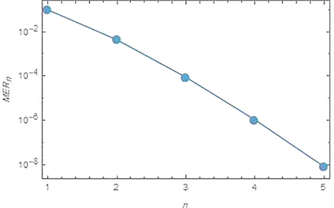
In order to examine the accuracy for the approximate solutions obtained by the proposed methods for Eq. (24) and since the exact solution is unknown, the maximal error remainder ${MER}_{n}$ will calculated. The error remainder function for problem 1 can be defined as

(36)

{ER}_{n} (x) = y_{n}^{″} (x) - 6 y_{n}^{2} (x) - x,

and the

{MER}_{n}

is:

(37)

{MER}_{n} = \max_{0.01 ⩽ x ⩽ 0.1} | {ER}_{n} (x) |,

Fig. 1 shows the logarithmic plots for ${MER}_{n}$ of the approximate solution obtained by the proposed iterative methods which indicates the efficiency of these methods. It can be seen that by increasing the iterations, the errors will be decreasing.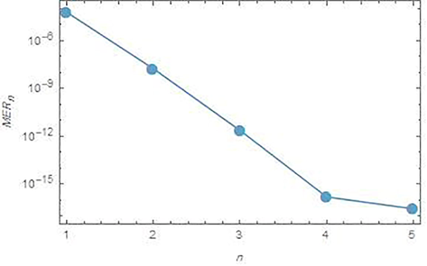

Logarithmic plots for the MER n versus n from 1 to 5, for problem 1.

Also, we have made a numerical comparison between the solutions obtained by the proposed methods, the Range-Kutta (RK4) and Euler methods. The comparison for problem1 is given in Fig. 2. It can be seen, a good agreement has achieved.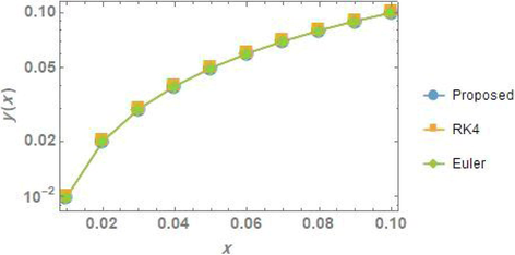

The comparison of the solutions for problem 1.

Problem 2:

The Painlevé equation II given by the following form (Hesameddini and Latifizadeh, 2012)

(38)

Y^{″} (x) = 2 y^{3} (x) + xy (x) + μ,

with the initial conditions:

y (0) = 1

and

y^{'} (0) = 0

. Eq. (39) will be solved by the three proposed iterative methods. The parameter

μ

in this work will be equal to 1.

Solving the problem 2 by the TAM:

In order to solve Eq. (39) by the TAM, we have the following form

(39)

L (y) = y^{″}, N (y) = 2 y^{3} + xy and g (x) = 1

The initial problem is

(40)

L (y_{0} (x)) = 0 with y_{0} (0) = 1 and y_{0}^{'} (0) = 0 .

The next problems can be found from the generalized iterative formula

L (y_{n + 1} (x)) + N (y_{n} (x)) = 0, y_{n + 1} (0) = 1 and y_{n + 1}^{'} (0) = 0 .

When evaluating the following initial problem (41), one can get

y_{0} (x) = 1 + \frac{x^{2}}{2} .

The first iteration

y_{1} (x)

can be found by solving

y_{1}^{″} (x) = 2 y_{1}^{2} (x) + {xy}_{1} (x) + 1 with y_{1} (0) = 1 and y_{1}^{'} (0) = 0 .

The solution will be

y_{1} (x) = 1 + \frac{3 x^{2}}{2} + \frac{x^{3}}{6} + \frac{x^{4}}{4} + \frac{x^{5}}{40} + \frac{x^{6}}{20} + \frac{x^{8}}{224} + \dots

Applying the same process for

y_{2}

as follows

y_{2}^{″} (x) = 2 y_{2}^{2} (x) + {xy}_{2} (x) + 1, with y_{2} (0) = 1 and y_{2}^{'} (0) = 0 .

By solving this problem, we have

y_{2} (x) = 1 + \frac{3 x^{2}}{2} + \frac{x^{3}}{6} + \frac{3 x^{4}}{4} + \frac{x^{5}}{8} + \frac{91 x^{6}}{180} + \frac{17 x^{7}}{210} + \frac{1409 x^{8}}{6720} + \frac{13 x^{9}}{288} + \frac{929 x^{10}}{16800} + \frac{38593 x^{11}}{3326400} + \frac{26683 x^{12}}{2217600} + \frac{1483 x^{13}}{655200} + \frac{6239 x^{14}}{3057600} + \frac{809 x^{15}}{2352000} + \frac{4583 x^{16}}{16128000} + \frac{2357 x^{17}}{60928000} + \frac{31273 x^{18}}{959616000} + \frac{37 x^{19}}{10944000} + \frac{3499 x^{20}}{1191680000} + \frac{109 x^{21}}{526848000} + \frac{81 x^{22}}{386355200} + \frac{3 x^{23}}{507781120} + \frac{x^{24}}{92323840} + \frac{x^{26}}{3652812800} + \dots

Continuing in this manner to get approximations up to $n = 5$ for $y_{n} (x)$ , but for brevity they are not listed.

Solving the problem 2 by the DJM:

Consider the Eq. (39) with initial conditions $y (0) = 1$ and $y^{'} (0) = 0$ .

Integrate both sides of Eq. (39) twice from $0$ to $x$ with using the given initial conditions, we obtain

(41)

y (x) = 1 + \frac{x^{2}}{2} + \int_{0}^{x} \int_{0}^{x} (2 y^{3} (τ) + τ y (τ)) d τ d τ,

and reducing the integration in Eq. (42) from double to single (Wazwaz, 2015), we achieve

(42)

y (x) = 1 + \frac{x^{2}}{2} + \int_{0}^{x} (x - τ) (2 y^{3} (τ) + τ y (τ)) d τ,

Therefore, we have the following recurrence relation

y_{0} = 1 + \frac{x^{2}}{2},

N (y_{n + 1}) = \int_{0}^{x} (x - τ) (2 y_{n}^{3} (τ) + τ y_{n} (τ)) d τ, n \in N \cup {0} .

By applying the DJM, we get $y_{0} = 1 + \frac{x^{2}}{2},$ $y_{1} = x^{2} + \frac{x^{3}}{6} + \frac{x^{4}}{4} + \frac{x^{5}}{40} + \frac{x^{6}}{20} + \frac{x^{8}}{224} + \dots,$ $y_{2} = \frac{x^{4}}{2} + \frac{x^{5}}{10} + \frac{41 x^{6}}{90} + \frac{17 x^{7}}{210} + \frac{197 x^{8}}{960} + \frac{13 x^{9}}{288} + \frac{929 x^{10}}{16800} + \frac{38593 x^{11}}{3326400} + \frac{26683 x^{12}}{2217600} + \frac{1483 x^{13}}{655200} + \frac{6239 x^{14}}{3057600} + \frac{809 x^{15}}{2352000} + \frac{4583 x^{16}}{16128000} + \frac{2357 x^{17}}{60928000} + \frac{31273 x^{18}}{959616000} + \frac{37 x^{19}}{10944000} + \frac{3499 x^{20}}{1191680000} + \frac{109 x^{21}}{526848000} + \frac{81 x^{22}}{386355200} + \frac{3 x^{23}}{507781120} + \frac{x^{24}}{92323840} + \frac{x^{26}}{3652812800} + \dots .$ Therefore, we continue to get approximations till $n = 5$ , for $y_{n} (x)$ but for brevity the terms are not listed.

Solving the problem 2 by the BCM:

Consider Eq. (39), by following the similar way in the DJM, we get the Eq. (43). So, let $y_{0} = 1 + \frac{x^{2}}{2}$ and $N (y_{n - 1}) = \int_{0}^{x} (x - τ) (2 y_{n - 1}^{3} (τ) + τ y_{n - 1} (τ)) d τ, n \in N$ .

The obtained solutions from the three proposed methods are same. Hence, as presented in the proof of the convergence for these methods in the previous section and by following similar procedure that presented for problem 1, the terms given by the series $\sum_{i = 0}^{\infty} v_{i} (x)$ in Eq. (21) satisfy the convergent conditions by evaluating the $β_{i}$ values for each iterative method, we get

(43)

\begin{matrix} β_{0} = \frac{v_{1}}{v_{0}} = 0.997421 < 1 \\ β_{1} = \frac{v_{2}}{v_{1}} = 0.983067 < 1 \\ β_{2} = \frac{v_{3}}{v_{2}} = 0.736222 < 1 \\ β_{3} = \frac{v_{4}}{v_{3}} = 0.500802 < 1 \\ β_{4} = \frac{v_{5}}{v_{4}} = 0.32419 < 1 \end{matrix}

where, the $β_{i}$ values for $i ⩾ 0$ and $0 < x ⩽ 1$ , are less than 1, so the proposed iterative methods are convergent.

Further investigation can be done, in order to examine the accuracy for the approximate solution for this problem; the error remainder function is evaluated:

(44)

{ER}_{n} (x) = y_{n}^{″} (x) - 2 y_{n}^{2} (x) - {xy}_{n} (x) - 1,

and the

{MER}_{n}

is:

(45)

{MER}_{n} = \max_{0.01 ⩽ x ⩽ 0.1} | {ER}_{n} (x) |,

Fig. 3 shows the logarithmic plots for

{MER}_{n}

of the approximate solution obtained by the proposed iterative methods which indicates the efficiency of these methods. Also, by increasing the iterations, the errors will be decreasing.

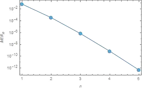
Logarithmic plots for the MER n versus n from 1 to 5, for problem 2.

The numerical comparison between the solutions obtained by the proposed methods, the Range-Kutta (RK4) and Euler methods for problem1 is given in Fig. 4, and good agreement is clearly obtained.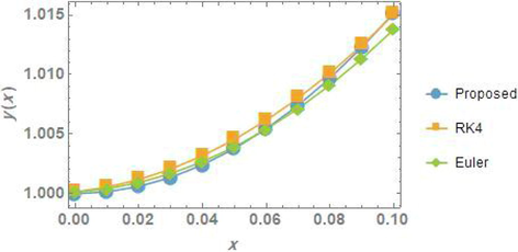

The comparison of the solutions for problem 2.

Problem 3:

The pendulum equation presented by the form (Duan, 2011)

(46)

y^{″} (x) + \sin y = 0,

with the given initial conditions:

y (0) = 0

and

y^{'} (0) = 1

, can be solved without linearization by using the approximation of

\sin y \approx y - \frac{1}{6} y^{3} + \frac{1}{120} y^{5}

as it used in (He, 1999). Hence, the pendulum equation (47) can be written by the following second order nonlinear ODE

(47)

y^{″} (x) + y - \frac{1}{6} y^{3} + \frac{1}{120} y^{5} = 0 .

The exact solution for Eq. (47) is expressed by the following Jacobi elliptic function

y = 2 \arcsin (\frac{1}{2} sn (x, \frac{1}{4}))

Solving the problem 3 by the TAM:

In order to solve the Pendulum equation given in Eq. (48) with the given conditions by the TAM, we have the following form

(48)

L (y) = y^{″}, N (y) = y - \frac{1}{6} y^{3} + \frac{1}{120} y^{5},

The initial problem is

(49)

L (y_{0} (x)) = 0 with y_{0} (0) = 0 and y_{0}^{'} (0) = 1 .

The next problems can be found from the generalized iterative formula

L (y_{n + 1} (x)) + N (y_{n} (x)) = 0, y_{n + 1} (0) = 0 and y_{n + 1}^{'} (0) = 1 .

By evaluating the initial problem (50), one can get

y_{0} (x) = x .

The first iteration

y_{1} (t)

can be found by solving

y_{1}^{″} (x) = - (y_{0} - \frac{1}{6} y_{0}^{3} + \frac{1}{120} y_{0}^{5}) {withy}_{1} (0) = 0 and y_{1}^{'} (0) = 1 .

The solution will be then

y_{1} (x) = x - \frac{x^{3}}{6} + \frac{x^{5}}{120} - \frac{x^{7}}{5040} .

Applying the same process for

y_{2}

as follows

y_{2}^{″} (x) = - (y_{1} - \frac{1}{6} y_{1}^{3} + \frac{1}{120} y_{1}^{5}) with y_{2} (0) = 0 and y_{2}^{'} (0) = 1 .

By solve this problem, we get

y_{2} (t) = x - \frac{x^{3}}{6} + \frac{x^{5}}{60} - \frac{x^{7}}{420} + \frac{127 x^{9}}{362880} - \frac{893 x^{11}}{19958400} + \frac{367 x^{13}}{70761600} - \frac{607 x^{15}}{1143072000} + \frac{56881 x^{17}}{1243662336000} - \frac{2521 x^{19}}{781861248000} + \frac{17 x^{21}}{92177326080} - \frac{22129 x^{23}}{2591207055360000} + \frac{17651 x^{25}}{55306395648000000} - \frac{61787 x^{27}}{6470848290816000000} + \frac{2021 x^{29}}{8981758653235200000} - \frac{73 x^{31}}{18002231783424000000} + \frac{13 x^{33}}{245294925978009600000} - \frac{x^{35}}{2211370923589632000000} + \frac{x^{37}}{519802247686127616000000} .

Continuing in this manner to get approximations up to

n = 5

for

y_{n} (t)

, but for brevity they are not listed.

Solving the problem 3 by the DJM:

Consider the Pendulum equation given in Eq. (48) with the given conditions $y (0) = 0$ and $y^{'} (0) = 1$ .

Integrating both sides of Eq. (48) twice from $0$ to $x$ , we get $y (t) = x - \int_{0}^{x} \int_{0}^{x} (y - \frac{1}{6} y^{3} + \frac{1}{120} y^{5}) d τ d τ,$ and reducing the integration in Eq. (51) from double to single (Wazwaz, 2015), we obtain

(50)

y (t) = x - \int_{0}^{x} (x - τ) (y - \frac{1}{6} y^{3} + \frac{1}{120} y^{5}) d τ,

Therefore, we have the following recurrence relation

y_{0} = x,

N (y_{n + 1}) = - \int_{0}^{x} (x - τ) (y_{n} - \frac{1}{6} y_{n}^{3} + \frac{1}{120} y_{n}^{3}) d τ, n \in N \cup {0} .

By applying the DJM, we get

y_{0} = x,

y_{1} = - \frac{x^{3}}{6} + \frac{x^{5}}{120} - \frac{x^{7}}{5040},

y_{2} = \frac{x^{5}}{120} - \frac{11 x^{7}}{5040} + \frac{127 x^{9}}{362880} - \frac{893 x^{11}}{19958400} + \frac{367 x^{13}}{70761600} - \frac{607 x^{15}}{1143072000} + \frac{56881 x^{17}}{1243662336000} - \frac{2521 x^{19}}{781861248000} + \frac{17 x^{21}}{92177326080} - \frac{22129 x^{23}}{2591207055360000} + \frac{17651 x^{25}}{55306395648000000} - \frac{61787 x^{27}}{6470848290816000000} + \frac{2021 x^{29}}{8981758653235200000} - \frac{73 x^{31}}{18002231783424000000} + \frac{13 x^{33}}{245294925978009600000} - \frac{x^{35}}{2211370923589632000000} + \frac{x^{37}}{519802247686127616000000} .

Therefore, we continue to get the other iterations till

n = 5

, for

y_{n} (x)

but for brevity the terms are not listed.

Solving the problem 3 by the BCM:

Consider Eq. (48), by applying the same way as in the DJM, we get the Eq. (52). So, let $y_{0} = x$ and $N (y_{n - 1}) = - \int_{0}^{x} (x - τ) (y_{n - 1} - \frac{1}{6} y_{n - 1}^{3} + \frac{1}{120} y_{n - 1}^{3}) d τ, n \in N$ .By applying the BCM, we obtain: $y_{0} = x,$ $y_{1} = x - \frac{x^{3}}{6} + \frac{x^{5}}{120} - \frac{x^{7}}{5040},$ $y_{2} = x - \frac{x^{3}}{6} + \frac{x^{5}}{60} - \frac{x^{7}}{420} + \frac{127 x^{9}}{362880} - \frac{893 x^{11}}{19958400} + \frac{367 x^{13}}{70761600} - \frac{607 x^{15}}{1143072000} + \frac{56881 x^{17}}{1243662336000} - \frac{2521 x^{19}}{781861248000} + \frac{17 x^{21}}{92177326080} - \frac{22129 x^{23}}{2591207055360000} + \frac{17651 x^{25}}{55306395648000000} - \frac{61787 x^{27}}{6470848290816000000} + \frac{2021 x^{29}}{8981758653235200000} - \frac{73 x^{31}}{18002231783424000000} + \frac{13 x^{33}}{245294925978009600000} - \frac{x^{35}}{2211370923589632000000} + \frac{x^{37}}{519802247686127616000000}$

We continue to get the other approximations till $n = 5$ , for brevity they are not listed.

The obtained solutions by the three proposed methods are equal to each other. Hence, as presented in the proof of the convergence in the previous section, the terms given by the series $\sum_{i = 0}^{\infty} v_{i} (x)$ in Eq. (21) satisfy the convergent conditions by evaluating the $β_{i}$ values for each iterative method, we get

(51)

\begin{matrix} β_{0} = \frac{v_{1}}{v_{0}} = 0.114522 < 1 \\ β_{1} = \frac{v_{2}}{v_{1}} = 0.0358901 < 1 \\ β_{2} = \frac{v_{3}}{v_{2}} = 0.019054 < 1 \\ β_{3} = \frac{v_{4}}{v_{3}} = 0.0114183 < 1 \\ β_{4} = \frac{v_{5}}{v_{4}} = 0.00760755 < 1 \end{matrix}

where, the

β_{i}

values for

i ⩾ 0

and

0 < x ⩽ 1

, are less than 1, so the proposed iterative methods are convergent.

To examine the accuracy of the obtained approximate solution for this problem, the error remainder function is evaluated

(52)

{ER}_{n} (x) = y_{n}^{″} (x) + y_{n} (x) - \frac{1}{6} y_{n}^{3} (x) + \frac{1}{120} y_{n}^{5} (x),

and the

{MER}_{n}

is:

(53)

{MER}_{n} = \max_{0 ⩽ x ⩽ 1} | {ER}_{n} (x) |,

Fig. 5 shows the logarithmic plots for

{MER}_{n}

of the approximate solution obtained by the proposed iterative methods which indicates the efficiency of these methods. Moreover, by increasing the iterations, the errors will be decreasing.

Logarithmic plots for the MER n versus n from 1 to 5, for problem 3.

In addition, the numerical comparison between the solutions obtained by the proposed methods, exact solution, the Range-Kutta (RK4) and Euler methods for problem 3 is presented in Fig. 6. The agreement between the solutions can be clearly seen.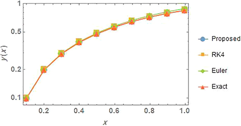

The comparison of the solutions for problem 3.

Problem 4:

The nonlinear reactive transport model is given in the following form (Ellery and Simpson, 2011):

(54)

y^{″} (x) - Py (x) - \frac{Ay (x)}{B + y (x)} = 0,

with the given boundary conditions:

y^{'} (0) = 0

and

y (1) = 1

, we select the values for the parameters

P = 0, A = 1

and

B = 2

as given in (Ellery and Simpson, 2011). The nonlinear second order ODE (56) will be

(55)

y^{″} (x) = \frac{y (x)}{2 + y (x)},

After doing a simple manipulation for Eq. (57), we have

(56)

y^{″} (x) + \frac{1}{2} y (x) y^{″} (x) - \frac{1}{2} y (x) = 0,

with the following initial conditions

y (0) = a

and

y^{'} (0) = 0

, where the unknown constant a will be evaluated later from the given boundary condition

y (1) = 1

Solving the problem 4 by the TAM:

In order to solve the Eq. (58) with the given initial conditions by the TAM, we have the following form

(57)

L (y) = y^{″}, N (y) = \frac{1}{2} y (x) y^{″} (x) - \frac{1}{2} y (x),

The initial problem is

(58)

L (y_{0} (x)) = 0 with y_{0} (0) = a and y_{0}^{'} (0) = 0 .

The next problems can be found from the generalized iterative formula

L (y_{n + 1} (x)) + N (y_{n} (x)) = 0, y_{n + 1} (0) = a and y_{n + 1}^{'} (0) = 0 .

By solving the initial problem (60), one can get

y_{0} (x) = a .

The first iteration

y_{1} (x)

can be found by solving

y_{1}^{″} (x) = - \frac{1}{2} y_{0} (x) y_{0}^{″} (x) + \frac{1}{2} y_{0} (x) with y_{1} (0) = a and y_{1}^{'} (0) = 0 .

The solution will be

y_{1} (x) = a + \frac{{ax}^{2}}{4} .

Applying the same process for

y_{2}

, we have

y_{2}^{″} (x) = - \frac{1}{2} y_{1} (x) y_{1}^{″} (x) + \frac{1}{2} y_{1} (x) with y_{2} (0) = a and y_{2}^{'} (0) = 0 .

By solving this problem, we obtain

y_{2} (x) = a + \frac{{ax}^{2}}{4} - \frac{a^{2} x^{2}}{8} + \frac{{ax}^{4}}{96} - \frac{a^{2} x^{4}}{192} .

Also, $y_{3}$ can be found by solving the problem

$y_{3}^{″} (x) = - \frac{1}{2} y_{2} (x) y_{2}^{″} (x) + \frac{1}{2} y_{2} (x)$ with $y_{3} (0) = a$ and $y_{3}^{'} (0) = 0$ , we get $y_{3} (x) = a + \frac{{ax}^{2}}{4} - \frac{a^{2} x^{2}}{8} + \frac{a^{3} x^{2}}{16} + \frac{{ax}^{4}}{96} - \frac{a^{2} x^{4}}{64} + \frac{a^{3} x^{4}}{128} - \frac{a^{4} x^{4}}{768} + \frac{{ax}^{6}}{5760} - \frac{a^{2} x^{6}}{1440} + \frac{7 a^{3} x^{6}}{11520} - \frac{7 a^{4} x^{6}}{46080} - \frac{a^{2} x^{8}}{86016} + \frac{a^{3} x^{8}}{86016} - \frac{a^{4} x^{8}}{344064} .$ Continuing in this manner to get the fourth and fifth approximations but for brevity they are not listed.

Solving problem 4 by the DJM:

Consider the Eq. (58) with the initial conditions $y (0) = a$ and $y^{'} (0) = 0$ .

Integrating both sides of Eq. (58) twice from $0$ to x, we get

(59)

y (x) = a + \int_{0}^{x} \int_{0}^{x} (- \frac{1}{2} y (τ) y^{″} (τ) + \frac{1}{2} y (τ)) d τ d τ,

and reducing the integration in Eq. (61) from double to single (Wazwaz, 2015), we obtain

(60)

y (x) = a + \int_{0}^{x} (x - τ) (- \frac{1}{2} y (τ) y^{″} (τ) + \frac{1}{2} y (τ)) d τ .

Therefore, we have the following recurrence relation

\begin{matrix} y_{0} = a, \\ N (y_{n + 1}) = \int_{0}^{x} (x - τ) (- \frac{1}{2} y_{n} (τ) y_{n}^{″} (τ) + \frac{1}{2} y_{n} (τ)) d τ, n \in N \cup {0} . \end{matrix}

By applying the DJM, we get

\begin{matrix} y_{0} = a, \\ y_{1} = \frac{{ax}^{2}}{4}, \\ y_{2} = - \frac{1}{8} a^{2} x^{2} + \frac{{ax}^{4}}{96} - \frac{a^{2} x^{4}}{192}, \\ y_{3} = \frac{a^{3} x^{2}}{16} - \frac{a^{2} x^{4}}{96} + \frac{a^{3} x^{4}}{128} - \frac{a^{4} x^{4}}{768} + \frac{{ax}^{6}}{5760} - \frac{a^{2} x^{6}}{1440} + \frac{7 a^{3} x^{6}}{11520} - \frac{7 a^{4} x^{6}}{46080} - \frac{a^{2} x^{8}}{86016} + \frac{a^{3} x^{8}}{86016} - \frac{a^{4} x^{8}}{344064} . \end{matrix}

Therefore, we continue to get the other approximations till

n = 5

for

y_{n} (t)

, but for brevity they are not listed.

Solving the problem 4 by the BCM:

Consider Eq. (58), by followed the same way as in the DJM, we get the Eq. (62). So, let $y_{0} = a$ and $N (y_{n - 1}) = \int_{0}^{x} (x - τ) (- \frac{1}{2} y_{n - 1} (τ) y_{n - 1}^{″} (τ) + \frac{1}{2} y_{n - 1} (τ)) d τ, n \in N$ .

By applying the BCM, we obtain:

(61)

\begin{matrix} y_{0} = a, \\ y_{1} = a + \frac{{ax}^{2}}{4}, \\ y_{2} = a + \frac{{ax}^{2}}{4} - \frac{a^{2} x^{2}}{8} + \frac{{ax}^{4}}{96} - \frac{a^{2} x^{4}}{192}, \\ y_{3} = a + \frac{{ax}^{2}}{4} - \frac{a^{2} x^{2}}{8} + \frac{a^{3} x^{2}}{16} + \frac{{ax}^{4}}{96} - \frac{a^{2} x^{4}}{64} + \frac{a^{3} x^{4}}{128} - \frac{a^{4} x^{4}}{768} + \frac{{ax}^{6}}{5760} - \frac{a^{2} x^{6}}{1440} + \frac{7 a^{3} x^{6}}{11520} - \frac{7 a^{4} x^{6}}{46080} - \frac{a^{2} x^{8}}{86016} + \frac{a^{3} x^{8}}{86016} - \frac{a^{4} x^{8}}{344064} . \end{matrix}

We continue to get the approximations till

n = 5

, for brevity they are not listed.

The value of a is evaluated by using the given boundary condition $y (1) = 1$ , so we have $a = 0.8466736340782172$ . Now, we can find the $β_{i}$ values in order to prove the convergence condition. Hence, the terms of the series $\sum_{i = 0}^{\infty} v_{i} (x)$ given in Eq. (21), we get

(62)

\begin{matrix} β_{0} = \frac{v_{1}}{v_{0}} = 0.397909 < 1 \\ β_{1} = \frac{v}{v_{1}} = 0.404609 < 1 \\ β_{2} = \frac{v_{3}}{v_{2}} = 0.411597 < 1 \\ β_{3} = \frac{v_{4}}{v_{3}} = 0.407664 < 1 \\ β_{4} = \frac{v_{5}}{v_{4}} = 0.40779 < 1 \end{matrix}

where, the

β_{i}

values for

i ⩾ 0

and

0 < x ⩽ 1

, are less than 1, so the proposed iterative methods are convergent.

To examine the accuracy for the approximate solution for this problem; the error remainder function is calculated

(63)

{ER}_{n} (x) = y_{n}^{″} (x) + \frac{1}{2} y_{n} (x) y_{n}^{″} (x) - \frac{1}{2} y_{n} (x),

and the

{MER}_{n}

is:

(64)

{MER}_{n} = \max_{0 ⩽ x ⩽ 1} | {ER}_{n} (x) |,

Fig. 7 shows the logarithmic plots for ${MER}_{n}$ of the approximate solution obtained by the proposed iterative methods which indicates the methods are reliable and effective. Also, by increasing the iterations, the errors will be decreasing.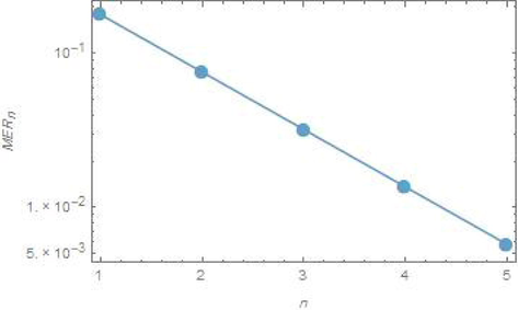

Logarithmic plots for the MER n versus n from 1 to 5, for problem 4.

Moreover, the numerical comparison between the solutions obtained by the proposed methods, the Range-Kutta (RK4) and Euler methods for problem 4 is presented in Fig. 8 and a good agreement can be clearly seen.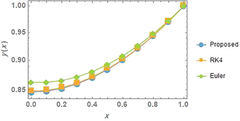

The comparison of the solutions for problem 4.

Problem 5:

The temperature distribution equation in a uniformly thick rectangular fin radiation to free space is given in the following form (Mohyud-Din et al., 2017)

(65)

y^{″} (x) - y^{4} (x) = 0,

with the given boundary conditions:

y^{'} (0) = 0

and

y (1) = 1

The Eq. (66) will be solved by the three iterative methods with the initial conditions $y (0) = a$ and $y^{'} (0) = 0$ , where the unknown constant a will be evaluated later from the given boundary condition $y (1) = 1$ . The parameter ε affects on the obtained solution will be seen numerically later.

Solving the problem 5 by the TAM:

In order to solve the Eq. (66) with the initial conditions by the TAM, we have the following form

(66)

L (y) = y^{″}, N (y) = y^{4} (x),

The initial problem is

(67)

L (y_{0} (x)) = 0 with y_{0} (0) = a and y_{0}^{'} (0) = 0 .

The next problems can be found from the generalized iterative formula

L (y_{n + 1} (x)) + N (y_{n} (x)) = 0, y_{n + 1} (0) = a and y_{n + 1}^{'} (0) = 0 .

By solving the initial problem (68), one can get

y_{0} (x) = a .

The first iteration

y_{1} (x)

can be found by solving

$y_{1}^{″} (x) = ∊ y_{0}^{4} (x)$ with $y_{1} (0) = a$ and $y_{1}^{'} (0) = 0$ .The solution will be $y_{1} (x) = a + \frac{1}{2} a^{4} x^{2} ∊ .$ Applying the same process for $y_{2}$ as follows $y_{2}^{″} (x) = y_{1}^{4} (x) with y_{2} (0) = a and y_{2}^{'} (0) = 0 .$ We solve this problem, we get $y_{2} (x) = a + \frac{1}{2} a^{4} x^{2} + \frac{1}{6} a^{7} x^{4} ∊^{2} ∊ + \frac{1}{20} a^{10} x^{6} ∊^{3} + \frac{1}{112} a^{13} x^{8} ∊^{4} + \frac{a^{16} x^{10} ∊^{5}}{1440} .$ Continuing in this manner to get the other approximations till $n = 5$ , but for brevity the evaluated terms are not listed.

Solving the problem 5 by the DJM:

Consider the Eq. (66) with the initial conditions $y (0) = a$ and $y^{'} (0) = 0$ .

Integrating both sides of Eq. (66) twice from $0$ to x, we get x

(68)

y (x) = a + \int_{0}^{x} \int_{0}^{x} (y^{4} (τ)) d τ d τ,

and reducing the integration in Eq. (69) from double to single (Wazwaz, 2015), we have

(69)

y (x) = a + \int_{0}^{x} (x - τ) (y^{4} (τ)) d τ .

Hence, we have the following recurrence relation

\begin{matrix} y_{0} = a, \\ N (y_{n + 1}) = \int_{0}^{x} (x - τ) (∊ y^{4} (τ)) d τ, n \in N \cup {0} . \end{matrix}

By applying the DJM, we get

(70)

\begin{matrix} y_{0} = a, \\ y_{1} = \frac{1}{2} a^{4} x^{2} ∊, \\ y_{2} = \frac{1}{6} a^{7} x^{4} ∊^{2} + \frac{1}{20} a^{10} x^{6} ∊^{3} + \frac{1}{112} a^{13} x^{8} ∊^{4} + \frac{a^{16} x^{10} ∊^{5}}{1440} . \end{matrix}

Therefore, we continue to get the other approximations till

n = 5

, for

y_{n} (x)

but the terms are not listed.

Solving the problem 5 by the BCM:

Consider Eq. (66), by applying the same procedure as in the DJM, we get the Eq. (70). So, let $y_{0} = a$ and $N (y_{n - 1}) = \int_{0}^{x} (x - τ) (y_{n - 1}^{4} (τ)) d τ, n \in N$ .

Applying the BCM, we obtain: $\begin{matrix} y_{0} = a, \\ y_{1} = a + \frac{1}{2} a^{4} x^{2} ∊, \\ y_{2} = a + \frac{1}{2} a^{4} x^{2} ∊ + \frac{1}{6} a^{7} x^{4} ∊^{2} + \frac{1}{20} a^{10} x^{6} ∊^{3} + \frac{1}{112} a^{13} x^{8} ∊^{4} + \frac{a^{16} x^{10} ∊^{5}}{1440} . \end{matrix}$

We continue to get the approximations till $n = 5$ , for brevity they are not listed.

The value of $a$ is obtained by using the given boundary condition $y (1) = 1$ for several values of a depends on the values of $∊$ . So, at $∊ = 0.1$ we get $a = 0.9568205007628632$ . Now, we can find the $β_{i}$ values in order to prove the convergence condition. Hence, the terms of the series $\sum_{i = 0}^{\infty} v_{i} (x)$ given in Eq. (21), we have

(71)

\begin{matrix} β_{0} = \frac{v_{1}}{v_{0}} = 0.0697115 < 1 \\ β_{1} = \frac{v_{2}}{v_{1}} = 0.0243227 < 1 \\ β_{2} = \frac{v_{3}}{v_{2}} = 0.0111531 < 1 \\ β_{3} = \frac{v_{4}}{v_{3}} = 0.00621257 < 1 \\ β_{4} = \frac{v_{5}}{v_{4}} = 0.00394466 < 1 \end{matrix}

where, the

β_{i}

values for

i ⩾ 0

and

0 < x ⩽ 1

, are less than 1, so the proposed iterative methods are convergent.

To examine the accuracy for the approximate solution for this problem; the error remainder function is ${ER}_{n} (x) = y_{n}^{″} (x) - ∊ y_{n}^{4} (x),$

and the ${MER}_{n}$ is:

(72)

{MER}_{n} = \max_{0 ⩽ x ⩽ 1} | {ER}_{n} (x) |,

Fig. 9 shows the logarithmic plots for ${MER}_{n}$ of the approximate solution obtained by the proposed iterative methods, it can be seen that by increasing the iterations, the errors will be decreasing.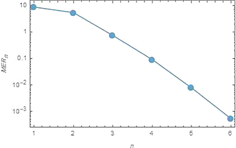

Logarithmic plots for the MER n versus n from 1 to 5, for problem 5.

The numerical comparison between the solutions obtained by the proposed methods, the Range-Kutta (RK4) and Euler methods for problem 5 is given in Fig. 10, once again a good agreement between the solution can be noticed.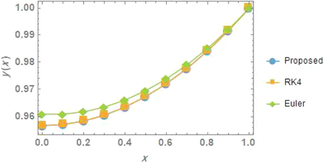

The comparison of the solutions for problem 5.

Moreover, we have plotted the effect of $\in$ for different values given in Fig. 11.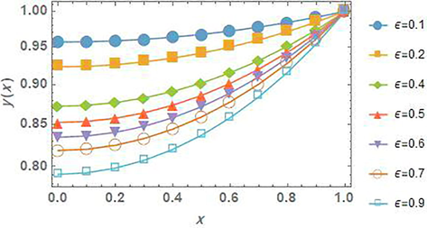

The numerical affections of ∈ values for problem 5.

Problem 6:

The motion equation for a system of mass with serial linear and nonlinear stiffness on a frictionless contact surface is presented by (Ganji and Babazadeh, 2009):

(73)

(1 + 0.1365 y^{2}) y^{″} + 0.2730 y {(y^{'})}^{2} + 4.5454 y + 2.2727 y^{3} = 0,

For more details for this model, we refer the reader to (Ganji and Babazadeh, 2009). Eq. (74) can be manipulated to get nonlinear the second order ODE

(74)

y^{″} + 0.1365 y^{2} y^{″} + 0.2730 y {(y^{'})}^{2} + 4.5454 y + 2.2727 y^{3} = 0,

with the initial conditions:

y = 0.5

and

y^{'} = 0

x = 0

Solving the problem 6 by the TAM:

In order to solve Eq. (75) with the initial conditions by the TAM, we have the following operators

(75)

\begin{matrix} L (y) = y^{″}, \\ N (y) = - (0.1365 y^{2} y^{″} + 0.2730 y {(y^{'})}^{2} + 4.5454 y + 2.2727 y^{3}) \end{matrix}

The initial problem is

(76)

L (y_{0}) = 0 with y_{0} (0) = 0.5 and y_{0}^{'} (0) = 0 .

The next problems can be found from the generalized iterative formula

$L (y_{n + 1}) + N (y_{n}) = 0, y_{n + 1} (0) = 0.5$ and $y_{n + 1}^{'} (0) = 0$ .

Solving the initial problem (77), one can get $y_{0} = 0.5 .$

The first iteration $y_{1} (x)$ can be found by solving

$y_{1}^{″} = - (0.1365 y_{0}^{2} y_{0}^{″} + 0.2730 y_{0} {(y_{0}^{'})}^{2} + 4.5454 y_{0} + 2.2727 y_{0}^{3})$ with $y_{1} (0) = 0.5$ and $y_{1}^{'} (0) = 0$ .

The solution will be $y_{1} = 0.5 - 1.27839375 x^{2} .$ Applying the same process for $y_{2}$ as follows

$y_{2}^{″} = - (0.1365 y_{1}^{2} y_{1}^{″} + 0.2730 y_{1} {(y_{1}^{'})}^{2} + 4.5454 y_{1} + 2.2727 y_{1}^{3})$ with $y_{2} (0) = 0.5$ and $y_{2}^{'} (0) = 0$ .

We solve this problem and then we have $y_{2} = 0.5 - 1.23476856328125 x^{2} + 0.5542817560763965 x^{4} - 0.09065096778687438 x^{6} + 0.08479065714299731 x^{8} .$ Continuing in this manner to get other approximations till $n = 5$ ; but for brevity they are not listed.

Solving problem 6 by the DJM:

Consider Eq. (77) with the initial conditions $y (0) = 0.5$ and $y^{'} (0) = 0$ .

Integrating both sides of Eq. (77) twice from $0$ to x, we get

(77)

y = 0.5 - \int_{0}^{x} \int_{0}^{x} (0.1365 y^{2} y^{″} + 0.2730 y {(y^{'})}^{2} + 4.5454 y + 2.2727 y^{3}) d τ d τ,

and reducing the integration in Eq. (78) from double to single (Wazwaz, 2015), we achieve

(78)

y = 0.5 - \int_{0}^{x} (x - τ) (0.1365 y^{2} y^{″} + 0.2730 y {(y^{'})}^{2} + 4.5454 y + 2.2727 y^{3}) d τ .

Hence, we have the following recurrence relation

\begin{matrix} y_{0} = 0.5, \\ N (y_{n + 1}) = - \int_{0}^{x} (x - τ) (0.1365 y_{n}^{2} y_{n}^{″} + 0.2730 y_{n} {(y_{n}^{'})}^{2} + 4.5454 y_{n} + 2.2727 y_{n}^{3}) d τ, n \in N \cup {0} . \end{matrix}

By applying the DJM, we get $\begin{matrix} y_{0} = 0.5, \\ y_{1} = - 1.27839375 x^{2}, \\ y_{2} = 0.04362518671875004 x^{2} + 0.5542817560763965 x^{4} - 0.09065096778687438 x^{6} + 0.08479065714299731 x^{8} . \end{matrix}$ Therefore, we continue to get approximations till $n = 5$ for $y_{n}$ , but the terms are not listed.

Solving the problem 6 by the BCM:

Consider Eq. (75), by following similar way used in the DJM, we get the Eq. (79). So, let $y_{0} = a$ and $N (y_{n - 1}) = - \int_{0}^{x} (x - τ) (0.1365 y_{n - 1}^{2} y_{n - 1}^{″} + 0.2730 y_{n - 1} {(y_{n - 1}^{'})}^{2} + 4.5454 y_{n - 1} + 2.2727 y_{n - 1}^{3}) d τ, n \in N$ .Applying the BCM, we obtain:

(79)

\begin{matrix} y_{0} = 0.5, \\ y_{1} = 0.5 - 1.27839375 x^{2}, \\ y_{2} = 0.5 - 1.23476856328125 x^{2} + 0.5542817560763965 x^{4} - 0.09065096778687438 x^{6} + 0.08479065714299731 x^{8} . \end{matrix}

We continue to get the approximations till

n = 5

, for brevity they are not listed.

Now, the $β_{i}$ values are evaluated in order to prove the convergence condition. Hence, the terms of the series $\sum_{i = 0}^{\infty} v_{i} (x)$ given in Eq. (21), we have

(80)

\begin{matrix} β_{1} = \frac{v_{2}}{v_{1}} = 0.378314 < 1 \\ β_{2} = \frac{v_{3}}{v_{2}} = 0.190321 < 1 \\ β_{3} = \frac{v_{4}}{v_{3}} = 0.0927949 < 1 \\ β_{4} = \frac{v_{5}}{v_{4}} = 0.0772565 < 1 \end{matrix}

where, the

β_{i}

values for

i ⩾ 1

and

0 < x ⩽ 1

, are less than 1, so the proposed iterative methods are convergent.

To examine the accuracy for the approximate solution for this problem; the error remainder function is

(81)

{ER}_{n} (x) = y_{n}^{″} (x) + 0.1365 y_{n}^{2} (x) y_{n}^{″} (x) + 0.273 y_{n} (x) {(y_{n}^{'} (x))}^{2} + 4.5454 y_{n} (x) + 2.2727 y_{n}^{3} (x),

and the

{MER}_{n}

is:

(82)

{MER}_{n} = \max_{0 ⩽ x ⩽ 1} | {ER}_{n} (x) |,

Fig. 12 shows the logarithmic plots for ${MER}_{n}$ of the approximate solution obtained by the proposed iterative methods, also, by increasing the iterations, the errors will be decreasing.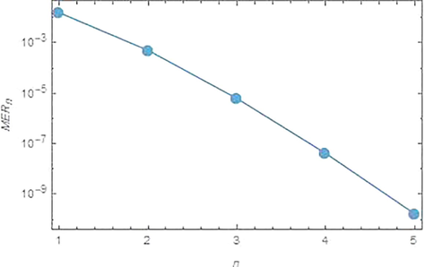

Logarithmic plots for the MER n versus n from 1 to 5, for problem 6.

The numerical comparison between the solutions obtained by the proposed methods, the Range-Kutta (RK4) and Euler methods for problem 6 is presented in Fig. 13.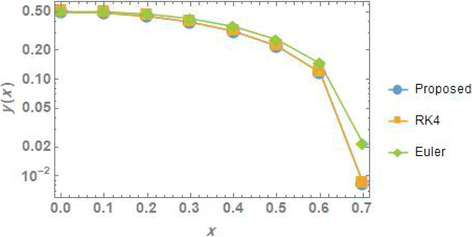

The comparison of the solutions for problem 6.

In Table 1, the convergence rate (CR) for all problems was estimated by using the following formula $ρ = \frac{\log (\frac{{MER}_{4}}{{MER}_{3}})}{\log (\frac{{MER}_{3}}{{MER}_{2}})},$

Table 1 The rate of convergence for the six problems.

Methods	Problem 1	Problem 2	Problem 3	Problem 4	Problem 5	Problem 6
The CR	1.03613	1.10076	1.13879	1.	1.14431	1.05231

Linear convergent has been achieved in all methods i.e. $ρ ≃ 1$ .

5 Conclusion

In our study of this paper, we have successfully used the TAM, DJM and BCM to solve several problems contain nonlinear second order ODEs that arising in physics problems. Each solution has been obtained in a series form. Then we solved these problems by numerical methods which are the Rang-Kutta (RK4) and Euler methods. We compared the numerical results with approximate solutions and were in good agreement. We have used the calculations in this study by the aid of Mathematica®10.

Acknowledgement

The author would like to thank the anonymous referees, Managing Editor and Editor in Chief for their valuable suggestions.

References

AL-Jawary M.A., . A semi-analytical iterative method for solving nonlinear thin film flow problems. Chaos, Solitons Fractals. 2017;99:52-56.
[Google Scholar]
AL-Jawary M.A., AL-Qaissy H.R., . A reliable iterative method for solving Volterra integro-differential equations and some applications for the Lane-Emden equations of the first kind. Monthly Not. R. Astronomical Soc.. 2015;448:3093-3104.
[Google Scholar]
AL-Jawary M.A., Al-Razaq S.G., . A semi analytical iterative technique for solving Duffing equations. Int. J. Pure Appl. Math.. 2016;108(4):871-885.
[Google Scholar]
AL-Jawary, M.A., Hatif, S., 2017. A semi-analytical iterative method for solving differential algebraic equations Ain Shams Eng. J., (In Press).
AL-Jawary M.A., Raham R.K., . A semi-analytical iterative technique for solving chemistry problems. J. King Saud Univ.. 2017;29(3):320-332.
[Google Scholar]
AL-Jawary M.A., Radhi G.H., Ravnik J., . A semi-analytical method for solving Fokker-Planck’s equations. J. Assoc. Arab Univ. Basic Appl. Sci.. 2017;24:254-262.
[Google Scholar]
Bhalekar S., Daftardar-Gejji V., . Solving evolution equations using a new iterative method. Numer. Methods Partial Diff. Eq.. 2010;26(4):906-916.
[Google Scholar]
Bhalekar S., Daftardar-Gejji, . New iterative method: application to partial differential equations. Appl. Math. Comput.. 2008;203(2):778-783.
[Google Scholar]
Daftardar-Gejji V., Bhalekar S., . Solving fractional diffusion-wave equations using a new iterative method. Fractional Calculus Appl. Anal.. 2008;11(2):193-202.
[Google Scholar]
Daftardar-Gejji V., Bhalekar S., . Solving nonlinear functional equation using Banach contraction principle. Far East J. Appl. Math.. 2009;34(3):303-314.
[Google Scholar]
Daftardar-Gejji V., Jafari H., . An iterative method for solving nonlinear functional equations. J. Math. Anal. Appl.. 2006;316(2):753-763.
[Google Scholar]
Duan J., . New recurrence algorithms for the nonclassic Adomian polynomials. Comput. Math. Appl.. 2011;62:2961-2977.
[Google Scholar]
Ehsani F., Hadi A., Ehsani F., Mahdavi R., . An iterative method for solving partial differential equations and solution of Korteweg-de Vries equations for showing the capability of the iterative method. World Appl. Programming. 2013;3(8):320-327.
[Google Scholar]
Ellery A.J., Simpson M.J., . An analytical method to solve a general class of nonlinear reactive transport models. Chem. Eng. J.. 2011;169:313-318.
[Google Scholar]
Ganji D.D., Babazadeh H., . M. H. Jalaei,·H. Tashakkorian, Application of He’s variational iteration method for solving nonlinear BBMB equations and free vibration of systems. Acta Applicandae Mathematicae. 2009;106:359-367.
[Google Scholar]
He J., . Variational iteration method – a kind of non-linear analytical technique: some examples. Int. J. Non Linear Mech.. 1999;34:699-708.
[Google Scholar]
Hesameddini E., Latifizadeh H., . A reliable treatment of homotopy purturbation method for solving second Painlevé equations. Int. J. Res. Rev. Appl. Sci.. 2012;12(2):201-206.
[Google Scholar]
Hesameddini E., Peyrovi A., . The use of variational iteration method and homotopy perturbation method for Painlevé equation I. Appl. Math. Sci.. 2009;3(38):1861-1871.
[Google Scholar]
Joshi M.C., Bose R.K., . Some Topics in Nonlinear Functional Analysis. John Wiley and Sons; 1985.
Liao S.J., Chwang A.T., . Application of homotopy analysis method in nonlinear oscillations. J. Appl. Mech.. 1998;65(4):914-922.
[Google Scholar]
Mohyud-Din S.T., Sikander W., Khan U., Ahmed N., . Optimal variational iteration method for nonlinear problems. J. Assoc. Arab Univ. Basic Appl. Sci.. 2017;24:191-197.
[Google Scholar]
Odibat Z.M., . A study on the convergence of variational iteration method. Math. Comput. Modell.. 2010;51(9–10):1181-1192.
[Google Scholar]
Temimi H., Ansari A.R., . A new iterative technique for solving nonlinear second order multi-point boundary value problems. Appl. Math. Comput.. 2011;218(4):1457-1466.
[Google Scholar]
Temimi H., Ansari A.R., . A computational iterative method for solving nonlinear ordinary differential equations. LMS J. Comput. Marhematics. 2015;18(1):730-753.
[Google Scholar]
Wazwaz A.M., . A first course in integral equations. World Scientific Publishing Company; 2015.

Introduction

The basic concepts of three iterative methods

The basic idea for the TAM
The basic idea for the DJM
The basic idea of the Banach contraction method (BCM)

The convergence of the proposed iterative methods

Test problems

Conclusion

Fulltext Views
37

PDF downloads
22

View/Download PDF
Download Citations

BibTeX
RIS

Show Sections

[1] AL-Jawary M.A., . A semi-analytical iterative method for solving nonlinear thin film flow problems. Chaos, Solitons Fractals. 2017;99:52-56.
[Google Scholar]

[2] AL-Jawary M.A., AL-Qaissy H.R., . A reliable iterative method for solving Volterra integro-differential equations and some applications for the Lane-Emden equations of the first kind. Monthly Not. R. Astronomical Soc.. 2015;448:3093-3104.
[Google Scholar]

[3] AL-Jawary M.A., Al-Razaq S.G., . A semi analytical iterative technique for solving Duffing equations. Int. J. Pure Appl. Math.. 2016;108(4):871-885.
[Google Scholar]

[4] AL-Jawary, M.A., Hatif, S., 2017. A semi-analytical iterative method for solving differential algebraic equations Ain Shams Eng. J., (In Press).

[5] AL-Jawary M.A., Raham R.K., . A semi-analytical iterative technique for solving chemistry problems. J. King Saud Univ.. 2017;29(3):320-332.
[Google Scholar]

[6] AL-Jawary M.A., Radhi G.H., Ravnik J., . A semi-analytical method for solving Fokker-Planck’s equations. J. Assoc. Arab Univ. Basic Appl. Sci.. 2017;24:254-262.
[Google Scholar]

[7] Bhalekar S., Daftardar-Gejji V., . Solving evolution equations using a new iterative method. Numer. Methods Partial Diff. Eq.. 2010;26(4):906-916.
[Google Scholar]

[8] Bhalekar S., Daftardar-Gejji, . New iterative method: application to partial differential equations. Appl. Math. Comput.. 2008;203(2):778-783.
[Google Scholar]

[9] Daftardar-Gejji V., Bhalekar S., . Solving fractional diffusion-wave equations using a new iterative method. Fractional Calculus Appl. Anal.. 2008;11(2):193-202.
[Google Scholar]

[10] Daftardar-Gejji V., Bhalekar S., . Solving nonlinear functional equation using Banach contraction principle. Far East J. Appl. Math.. 2009;34(3):303-314.
[Google Scholar]

[11] Daftardar-Gejji V., Jafari H., . An iterative method for solving nonlinear functional equations. J. Math. Anal. Appl.. 2006;316(2):753-763.
[Google Scholar]

[12] Duan J., . New recurrence algorithms for the nonclassic Adomian polynomials. Comput. Math. Appl.. 2011;62:2961-2977.
[Google Scholar]

[13] Ehsani F., Hadi A., Ehsani F., Mahdavi R., . An iterative method for solving partial differential equations and solution of Korteweg-de Vries equations for showing the capability of the iterative method. World Appl. Programming. 2013;3(8):320-327.
[Google Scholar]

[14] Ellery A.J., Simpson M.J., . An analytical method to solve a general class of nonlinear reactive transport models. Chem. Eng. J.. 2011;169:313-318.
[Google Scholar]

[15] Ganji D.D., Babazadeh H., . M. H. Jalaei,·H. Tashakkorian, Application of He’s variational iteration method for solving nonlinear BBMB equations and free vibration of systems. Acta Applicandae Mathematicae. 2009;106:359-367.
[Google Scholar]

[16] He J., . Variational iteration method – a kind of non-linear analytical technique: some examples. Int. J. Non Linear Mech.. 1999;34:699-708.
[Google Scholar]

[17] Hesameddini E., Latifizadeh H., . A reliable treatment of homotopy purturbation method for solving second Painlevé equations. Int. J. Res. Rev. Appl. Sci.. 2012;12(2):201-206.
[Google Scholar]

[18] Hesameddini E., Peyrovi A., . The use of variational iteration method and homotopy perturbation method for Painlevé equation I. Appl. Math. Sci.. 2009;3(38):1861-1871.
[Google Scholar]

[19] Joshi M.C., Bose R.K., . Some Topics in Nonlinear Functional Analysis. John Wiley and Sons; 1985.

[20] Liao S.J., Chwang A.T., . Application of homotopy analysis method in nonlinear oscillations. J. Appl. Mech.. 1998;65(4):914-922.
[Google Scholar]

[21] Mohyud-Din S.T., Sikander W., Khan U., Ahmed N., . Optimal variational iteration method for nonlinear problems. J. Assoc. Arab Univ. Basic Appl. Sci.. 2017;24:191-197.
[Google Scholar]

[22] Odibat Z.M., . A study on the convergence of variational iteration method. Math. Comput. Modell.. 2010;51(9–10):1181-1192.
[Google Scholar]

[23] Temimi H., Ansari A.R., . A new iterative technique for solving nonlinear second order multi-point boundary value problems. Appl. Math. Comput.. 2011;218(4):1457-1466.
[Google Scholar]

[24] Temimi H., Ansari A.R., . A computational iterative method for solving nonlinear ordinary differential equations. LMS J. Comput. Marhematics. 2015;18(1):730-753.
[Google Scholar]

[25] Wazwaz A.M., . A first course in integral equations. World Scientific Publishing Company; 2015.

Three iterative methods for solving second order nonlinear ODEs arising in physics

Abstract

Keywords

Iterative methods

Approximate solution

Numerical solution

Runge-Kutta 4 method

Euler method

1 Introduction

2 The basic concepts of three iterative methods

2.1 The basic idea for the TAM

2.2 The basic idea for the DJM

2.3 The basic idea of the Banach contraction method (BCM)

3 The convergence of the proposed iterative methods

4 Test problems

5 Conclusion

Acknowledgement

References

Suggested read for related articles: