

Translate this page into:
Theoretical analysis of unstable segments of electrostatic spinning charged jet
⁎Corresponding author. zhyliang@dhu.edu.cn (Liang Zhiyong)
-
Received: ,
Accepted: ,
This article was originally published by Elsevier and was migrated to Scientific Scholar after the change of Publisher.
Peer review under responsibility of King Saud University.
Abstract
The basic mechanism of electrospinning is the rapid whipping of charged liquid jets, undergoing a chaotic “whip” process, and eventually the formation of disordered reticular fibers is continuously deposited on the receiving device. Firstly, the physical model of jet whipping is studied, which is to be established the physical model of solvent evaporation on the surface of the jet. The Jeffreys model and the Voigt model are used to describe the viscoelastic model of the unstable generating end and the end, and the unstable dynamic model is constructed. Finally, the coupling control equation is obtained, which has certain theoretical guiding significance for the development of electrospinning process.
Keywords
Electrospinning
Viscoelastic behavior model
Solvent evaporation
Jeffreys model
Governing equation

1 Introduction
Under the action of the electric field force of the high voltage electrostatic field, the polymer solution forms a “Taylor cone” due to the interaction of electrostatic force and surface tension (Taylor, 1964). As the applied voltage increases, the solution overcomes the surface tension and viscous resistance from the tip of the Taylor cone. With a charged jet, the polymer jet evaporates and solidifies during the spraying process, and finally reaches the receiving device to form ultrafine fibers, and the diameter is generally between 5 nm and 1000 nm (Teo and Ramakrishna, 2006; Fang et al., 2010). As early as 1934, Formahals first described in detail the use of high-voltage static electricity to prepare nanofiber devices and applied for related patents. The research on jet is divided into three parts: “Taylor cone”, jet stability section and unstable section. The electrospinning process is complex and involves subject knowledge such as rheology, electrostatics, electrohydrodynamics and chemistry (Dacheng and du Zhongliang, 2003). The materials are widely used, from the initial filtration and reinforced composite materials to biomedicine and energy new areas such as high efficiency filtration, stent loading, battery separators and tissue engineering. So far, most of the electrospinning production has not yet reached the industrial production standard, but only stays in the laboratory stage, which has great application potential.
Environmental conditions (like relative humidity and temperature) are also important factors, which can affect the morphology of nanofibers (Cui et al., 2020). Generally, low relative humidity will accelerate the evaporation rate of solvent in the jet, which is conducive to the formation of thinner fibers. Temperature has two opposite effects on the average fiber diameter. An increase in temperature will accelerate the evaporation rate of the solvent, limiting further stretching of the jet. Low temperature reduces the viscosity of the solution and facilitates the formation of thinner fibers. Therefore, it is necessary to adjust the temperature and humidity of the environment reasonably to achieve the optimal electrospinning conditions.
Electrospinning technology is divided into solution electrospinning and melts electrospinning. Although both methods can prepare nanofibers, their respective technologies have shortcomings. The key problem is the lack of research on basic theory, so it is very difficult to guide the corresponding spinning process. Many models have been developed to simulate the jetting behavior of electrospinning. Hohman et al. (2001), Hohman et al. (2001) developed the “slim body” theory in the direct jet region and the curved region to consider the effects of viscoelastic force, surface tension and electric field force, but the effect of solvent volatilization on fiber formation was not considered. For the stable section of the jet, Feng (2002) simplifies the elongated body model of Newtonian fluid without considering the effects of solvent evaporation. For the unstable section of the jet, Fridrikh et al. (2003) analyzed Hohman’s whipping jet dynamics equation to obtain the scaling law, but did not consider the viscous force in the fiber diameter scaling law, ignoring the fluid's non-Newtonian fluid properties and solvent volatilization and elasticity. Yarin et al. (2001) proposed the Maxwell model to describe the viscoelastic properties of the jet in the unstable section, considering the effects of solvent evaporation and solidification, but did not analyze how RH affects the volatilization and stress state.
In addition, recent studies have been conducted by Topuz et al. (2021) focusing on the electrospinning parameters from practical and theoretical perspective. In this study, they explored the effect of the electrospinning parameters — namely polymer concentration, voltage, tip-to-collector distance and flow rate — and salt addition on the diameter, morphology, and spinnability of electrospun PI nanofibers. They also used molecular dynamic simulations to investigate the macromolecular mechanism of improved spinnability and fiber morphology in the presence of an ammonium salt. Therefore, the study of the basic theory of electrospinning is not only challenging, but also very necessary.
The purpose of this article is to use the existing theories, put them in the electrospinning jet and knead them together for analysis and research, and finally obtain the conversion control equation. The study mainly focuses on the research of the charged jet in the small segment. The author first carried out mathematical derivation, and then established the motion control equation of the variable segment jet. The charged jet in the unstable section is a relatively difficult part of theoretical research. The author combined many other models in the research process, such as Maxwell viscoelastic model, Voigt model and etc. The author’s theoretical derivation will provide certain theoretical guidance for the development of electrospinning technology.
2 Basic theory and assumptions
Firstly, only one commonly used solution is considered in the research, and other cases are temporarily not considered. In electrospinning, assuming that the liquid is weakly conductive, a “drain dielectric model” (Saville, 1997) is cited, the jet carries only the charge on the surface, and any internal charge quickly enters the surface. At the same time the fluid has sufficient dielectric to maintain an electric field tangent to the surface of the jet, the viscoelastic behavior of the polymer solution is described by a linear Maxwell rheological model, the electrospinning process begins with the needle, only a single jet is analyzed, regardless of the injection, which the flow splits into a secondary jet.
2.1 Mass conservation equation of jet
The mass conservation of the i-th cylinder in the unstable section of the jet is as shown in Eq. (1).
Ambient relative humidity (
) is defined as the ratio of the vapor pressure of water in air (
) to the saturated vapor pressure (
) of water at the same temperature and pressure. For a constant temperature (
), the evaporation rate (
) of the aqueous solution is proportional to (
) (Jayjock, 1994), as shown in Eq. (2).
The Nusselt number is a dimensionless heat transfer coefficient that describes the rate of heat transfer. By setting the Prandtl number to, we derive the arbitrary value of the Prandtl number correlation of Eq. (5) and obtain it as shown in Eq. (6).
Similar to formula (6), the correlation of sherwood numbers is used.
The mass transfer coefficient of the solution of the simultaneous (4)–(7) solution is as shown in the formula (8).
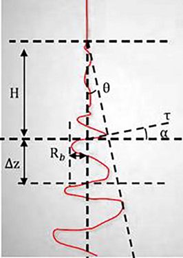
Single jet unstable section photo.
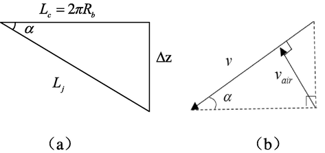
(a) The triangular relationship between
,
, and
. (b) the relationship between
and
.
Based on Figs. 1–2b, the relationship between
and
is as shown in Eq. (11).
Substituting the formula (11) into the formula (8), the expression for obtaining the mass transfer coefficient of the solution is as shown in the formulas (12) and (13).
The surface area of the i-th jet is as shown in Eq. (14).
The expression of the volatilization rate substituted by (3) is as shown in the formula (Yan, 2011).
Replace formula (13) with (15), that is,
If water is used as the solvent, the volatilization rate equation is a function of relative humidity (
), volume flow (
) of the i-th segment, and jet cross-section radius (
), as shown in Eq. (17).
For solvents other than water, it is reasonable to assume that the vapor pressure in the ambient air is zero due to ventilation around the rotating device. Therefore, the volatilization rate expression is as shown in the formula (18).
Equation (16) indicates that the volatilization of the jet surface is inseparable from the air cross velocity, jet radius, length, and helix angle, Eq. (17) shows that the volatilization of the solvent and the relative humidity (RH) of the solution have a great influence on the fiber diameter, The solvent volatilization indicating the surface of the whipped jet is a function of vapor pressure differential, jet flow, jet diameter and total jet length. The smaller the radius, the higher the local jet velocity, and the higher the volumetric surface area, the higher the solvent evaporation rate is.
2.2 Viscoelastic behavior model and constitutive equation of jet
Electrospinning is a typical viscoelastic fluid jet process. The viscoelastic force can significantly affect the stretching and deposition of the jet. The solution of the polymer solution has both viscous and elastic properties in the initial stage of the stable and unstable phases of the jet, in the deposition process, as the fiber volatilizes and solidifies; it has the properties of an elastic solid. Joseph describes the application of the Maxwell viscoelastic model in viscoelastic fluids (Bird et al., 1987), which describes the mechanical properties of viscoelastic bodies in a model formed by different combinations of elastic and viscous elements. Springs (elastic elements) are typically used to simulate elastic solids, and dampers (viscous elements) mimic viscous liquids, i.e. the viscous flow of macromolecular chains in fibrous materials.
For the elastic element as shown in Fig. 3 (a), the relationship between stress and strain is as shown in Eq. (19).
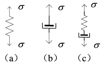
(a) A rigid spring represents an elastic element; (b) a damper represents a viscous element, (c) a Maxwell viscoelastic model.
For the viscous element as shown in Fig. 3 (b), the relationship between stress and strain is as shown in Eq. (20).
-
(1)
The Maxwell model is a rheological model used to describe viscoelastic fluids.
It is often used as a submodel to study multivariate combined rheological models. The viscoelastic model is shown in Fig. 3 (c). The model consists of a series of springs and dampers, where the spring rate is
, the damper viscosity is
, the spring and damper strains are
,
, the spring and damper stresses are
,
, respectively. The relationship between stress and strain of the spring and the damper in the case of series is as shown in Eq. (21).
The function expression of the strain rate of the Maxwell model is shown in Eq. (22).
Then the viscoelastic constitutive equation of the Maxwell model is shown in Eq. (23).
Equation (23) is the differential equation of stress and strain, that is, the constitutive equation of Maxwell。
The viscoelastic constitutive equation of the jet linearized one-dimension model is shown in Eq. (25).
The wave equation of the jet is shown in Eq. (26).
-
(2)
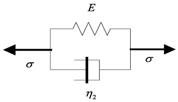
The Voigt model consists of a parallel connection of springs and dampers
As shown in Figs. 2–4 the Voigt model can better describe the creep phenomenon and elastic aftereffect of the fiber during the jet process, and can be applied to the end of the unstable segment of the jet to describe the volatilization and solidification of the fiber. In the model the force of the spring element is
, the force of the viscous unit is
and the total stress is added in parallel, so the viscoelastic physical model of the end of the unstable section of the jet is shown in Eq. (28).
Voigt model.
The strain ε and strain rate of the model spring and damper are designed to occur simultaneously, which is characterized by “elastic solid”. Therefore, the model is applied to the end of the jet, and the solvent volatilizes with the movement of the jet and finally solidifies into nanofiber.
The strain and strain rate of the model spring and damper are designed to occur simultaneously, which is characterized by “elastic solid”. Therefore, the model is applied to the end of the jet, and the solvent volatilizes with the movement of the jet and finally solidifies into nanofiber.
The end of the unstable segment of the jet belongs to the viscoelastic fluid and is therefore simulated by the Jeffreys model.
The damper and Voigt model are connected in series, as shown in Fig. 5. The total strain in the Jeffreys model is the strain of the damper and the Voigt model. The sum of the stresses of the two components is equal. In the Voigt model, not only the elastic deformation but also the viscous deformation of the damper, the Jeffreys model has viscoelastic properties.
and
are related to
partial differential equations such as (29) And (30) are shown.
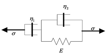
Jeffreys model.
The viscoelastic physical model of the end of the unstable segment of the jet obtained by the combination of Eqs. (29) and (30) is shown in (31).
3 Jet instability segment dynamics model
Based on the jet mass conservation equation and viscoelastic model established in the previous section, the following is mainly the force analysis of the unstable segment of the jet. The main forces of the jet during the “whipping” process are viscous force, applied electric field force, surface tension, air resistance and Gravity, through theoretical calculations, analyzes the influence of each force on the jet, and simplifies the force model. The electrospinning jet motion model is shown in Figs. 1–6. The model unit is made up of Maxwell model in series with each other, using spring to simulate elastic components, using a damper to represent the viscous element, all the mass and charge of the unit are concentrated on the sphere (approximate mass).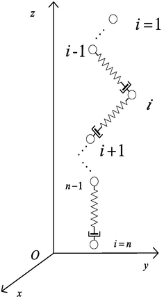
Viscoelastic model of jet instability section.
Use the subscript n to indicate the viscoelastic element section (i,i + 1) and the subscript d to indicate the (i − 1,i) segment of the viscoelastic element, as shown in Figs. 1–6. The distance between adjacent viscoelastic elements is as shown in Eqs. (33) and (34)
,
and
are the instantaneous normal stress, instantaneous dynamic viscosity and instantaneous relaxation time of the
-th segment of the jet unit respectively,
,
and
are the instantaneous normal stress, instantaneous dynamic viscosity and instantaneous relaxation time of the
-th segment. The instantaneous mass fraction (
) of the
-th segment, the initial mass (
) is shown in Eq. (36)
3.1 Viscoelastic force
Solvent volatilization is considered in the unstable section of the jet
Therefore, the volume relaxation factor (
) is the ratio of the instantaneous volume of the jet to the initial volume, as shown in Eq. (39).
Then, in the
segment and the
segment of the jet unit, the instantaneous radii
and
are as shown in Eq. (40)
Then, for the mass point
, only the viscoelastic force of the adjacent mass point
and the mass point
, the viscoelastic force acting on the mass point
is as shown in the formula (43).
3.2 Surface tension
Surface tension is the resistance variable that the liquid itself produces in order to maintain its own morphological deformation, which hinders the change of the surface of the liquid. In the process of electrospinning, surface tension is one of the main forces that cause the jet to twist and rotate. Polymer liquid jet. The stretching increases the surface area and increases the surface energy
. For the particle
, the surface tensions
and
of the
and
segments are simultaneously applied, and the direction of the surface tension is the same as the axial direction of the segment. Then the
and
segments are correlated. The surface energy is as shown in Eq. (44).
Equation (40) is substituted into Eq. (44) to obtain the surface energy expression as shown in (45).
Where
is the surface tension coefficient of the polymer solution. The surface tension is the derivative of the surface energy
versus the length (
). According to the expression of the relationship between surface tension and surface energy the surface tensions
and
are as shown in Eq. (46)
In addition to the surface tension parallel to the cross section and perpendicular to the contour, the additional surface tension due to the bending of the charged liquid, and the line of action points to the center of the circle along the radial direction of the circle corresponding to the jet micro-element. Section
and
The radius of curvature corresponding to the segments is approximately equal, and the additional surface tension
is as shown in Eq. (47).
Where
is the radius of curvature corresponding to the
,
jet micro-element segment,
is the center of the curvature circle,
is the vector radius of the center of the circle. Therefore, the surface tension
of the particle
is as shown in Eq. (48).
3.3 Electric field force
The electric field force is the most important force for the formation of electrospun fibers. According to the electrical principle, the electric field force of charged particles in the electric field is
. In the electrospinning experiment, the electric field strength satisfies the tip-plate electric field distribution model (Coelho and Debeau, 1971). According to this model, the electric field distribution between the needle and the deposition plate is shown in Figs. 2–7. When the voltage applied between the needle and the deposition plate is
, Coelho (Zeng et al., 2005) analyzed the expression of the potential intensity as shown in Eq. (49)
The corresponding electric field strength expression is shown in Eq. (50).
The electric field strength at each point on the extension line of the polymer needle tip can be simplified to
Where is the equipotential elliptical polar angle of the equipotential surface, is the polar angle of the co-hyperbolic curve of the equipotential surface, is the distance between the polymer needle and the calculated point, and is the distance from the needle to the deposition plate, is the diameter of the needle. It can be seen from Eqs. (49) and (50) that the electric field strength increases with the increase of the applied voltage and decreases rapidly as the distance between the needle and the deposition plate increases.
At that time, the electric field strength at the position of the deposition plate was
.
In the viscous unit, the mass of the mass point is
, and the electric field force that the particle receives in the electric field is
Where represents the unit vector along the direction, the direction is vertically upward along the deposition plate, similarly , is the unit vector of , direction.
3.4 Coulomb force
Coulomb force is the interaction between two stationary point charges in a vacuum as shown in Eq. (54)
Since the charge property on the surface of the jet is the same, assuming that the mass of the mass
is
, the particle
is simultaneously subjected to the Coulomb force vector of all the particles on the jet to the mass
as shown in Eq. (56).
3.4 3.5 air resistance
The frictional resistance between the charged jet and the surrounding gas is divided into frictional resistance and pressure resistance. The mass
of the mass point
is
Where ρs is the unit density of the fiber, and the resistance
received by the mass point
is provided by the
and
segments of the jet micro-element, as shown in Eq. (59).
Where Cf is the frictional resistance coefficient, Cp is the pressure resistance coefficient, Atdi is the surface area of the
segment, Amdi is the maximum cross-sectional area of the
segment, ρair is the air density, vti is the axial relative velocity of the particle,
is the normal velocity. The relative speed at
is as shown in equation (61).
3.5 Gravity
The gravity received by the particle is shown in Eq. (63).
4 Control equation
According to Newton's second law, the force equation of the particle
can be obtained as follow
The main forces on the unstable section of the jet are: viscoelastic force, surface tension, electric field force, Coulomb force, resistance, gravity. Then the force received by the micro-body in the
segment is substituted (64) to obtain the viscoelastic element, Grande equation
The Euler equation for air is (Zeng et al., 2005)
5 Conclusion
The purpose of this article is to use the existing theories to knead them together in the unstable jet of electrospinning, conduct analysis and research, and finally obtain the coupled control equation. Several findings are listed below.
(1) In this paper the mass transfer coefficient equation of liquid and the evaporation rate equation of jet under different solvents are derived. The one-dimension model of jet viscoelastic linearization is established.
(2) For the first time, the Jeffrey’s model is used to describe the jet as both viscous and elastic at the end of the unstable section of the jet. The Voigt model describes the creep phenomenon and the elastic aftereffect of the unstable section of the jet, which will be used to study the structural performance of the unstable section of the jet.
(3) Stress analysis of the unstable section of the jet, theoretical calculation of viscoelastic force, surface tension, Coulomb force, electric field force, air resistance, and gravity based on the Maxwell viscoelastic model to establish the coupling of the unstable segment of the jet. The governing equations combined with the conclusion (1) will be numerically simulated in the next step of jet formation.
Acknowledgements
This work was partly supported by the Chang Jiang Youth Scholars Program of China and grants (51373033) from the National Natural Science Foundation of China to Prof. Xiaohong Qin, as well as “The Fundamental Research Funds for the Central Universities” and “DHU Distinguished Young Professor Program” to her. It also has the support of the Key grant Project of Chinese Ministry of Education (No 113027A). This work has also been supported by “Sailing Project” from Science and Technology Commission of Shanghai Municipality (14YF1405100) to Dr. Hongnan Zhang.
Declaration of Competing Interest
The authors declare that they have no known competing financial interests or personal relationships that could have appeared to influence the work reported in this paper.
References
- Proc. Roy. Soc. Lond. A-Math. Phy. Sci.. 1964;280(1382):383-397.
- Nanotechnology. 2006;17(14):89-106.
- Evolution of fiber morphology during electrospinning. J. Appl. Polym. Sci.. 2010;118(5):2553-2561.
- [Google Scholar]
- Formahals. A., 1934. USP 1975504.
- Wu Dacheng, du Zhongliang, Gao Xushan. Nanofibers. Beijing: Chemical Industry Press, 2003.
- Electrospun nanofiber membranes for wastewater treatment applications. Sep. Purif. Technol.. 2020;250:117116.
- [Google Scholar]
- Electrospinning and electrically forced jets. I. Stability theory. Phys. Fluids. 2001;13(8):2201-2220.
- [Google Scholar]
- Electrospinning and electrically forced jets. II. Applications. Phys. Fluids. 2001;13(8):2221-2236.
- [Google Scholar]
- The stretching of an electrified non-Newtonian jet: a model for electrospinning. Phys. Fluids. 2002;14(11):3912-3926.
- [Google Scholar]
- Controlling the fiber diameter during electrospinning. Phys. Rev. Lett.. 2003;90(14)
- [Google Scholar]
- Bending instability in electrospinning of nanofibers. J. Appl. Phys.. 2001;89(5):3018-3026.
- [Google Scholar]
- Nanofiber engineering of microporous polyimides through electrospinning: influence of electrospinning parameters and salt addition. Mater. Des.. 2021;198:109280.
- [Google Scholar]
- Electrohydrodynamics: the Taylor-Melcher Leaky dielectric model. Annu. Rev. Fluid Mech.. 1997;29(1):27-64.
- [Google Scholar]
- Back pressure modeling of indoor air concentration from volatilizing sources. Am. Ind. Hyg. Assoc. J.. 1994;55:230-235.
- [Google Scholar]
- Viscous Fluid Flow. New York: McGraw-Hill; 2006.
- Fundamentals of Fibre Formation. London: Wiley; 1976.
- Electospinning of Nanofibers: Analysis of Diameter Distribution and Process Dynamics for Control. Boston University, College of Engineering; 2011. p. :340.
- Dynamiccs of Polymeric Liquids (second ed.). New York: Wiley; 1987.
- Mixed Euler-Lagrange approach to modeling fiber motion in high speed air flow. Appl. Math. Model. 2005;29(3):253-262.
- [Google Scholar]
- Applied Fluid Mechanics (third ed.). Columbus: Merrill; 1990. p. :645.


