

Translate this page into:
The Marshall-Olkin extended inverted Kumaraswamy distribution: Theory and applications
⁎Corresponding author. usmanrana0331@gmail.com (Rana Muhammad Usman)
-
Received: ,
Accepted: ,
This article was originally published by Elsevier and was migrated to Scientific Scholar after the change of Publisher.
Peer review under responsibility of King Saud University.
Abstract
A new three parametric distribution is proposed and analyzed, termed as the Marshall-Olkin extended inverted Kumaraswamy (MOEIK) distribution. This generalization has some renowned sub models such as the Beta type II, the Lomax and the Fisk distribution, stated in literature. Study includes the basic properties of the observed probabilistic model. Explicit expressions for major mathematical properties of this distribution such as quantile function, complete and incomplete moments, entropies and moments of order statistic are derived. Maximum likelihood estimation method is used to estimate the parameters. For different parameter values, a number of simulation studies are conducted for different sample sizes and compare the performance of the MOEIK distribution. Three real life applications are provided to explain the potentiality and reliability of the extended distribution with confidence that the generalized model have wider applications in hydrology and the associated fields.
Keywords
Inverted Kumaraswamy distribution
Quantile function
Moment generating function
Order statistic
Maximum likelihood

1 Introduction
From last few decades researchers have greater intention toward the inversion of univariate probability models and their applicability under inverse transformation i.e. inverted beta (Dubey, 1970), inverse Rayleigh (Voda, 1972), inverse Gaussian (Folks and Chhikara, 1978), inverse Weibull (Calabria and Pulcini, 1990), inverted Burr type XII also called Burr type III (Al-Dayian, 1999), inverse Rayleigh (Rosaiah and Kantam, 2005), inverted exponential (Dey, 2007), inverse Lindley (Sharma et al., 2015) and many other distributions.
Since two-parameter Kumaraswamy distribution has much importance as a substitute of the beta distribution introduced by Kumaraswamy (1980) during the explanation of hydrological applications. He had found that numerous important distributions such as log normal distribution, normal distribution, beta distribution and many more do not have better fit on hydrological data i.e. daily stream flow data and rain fall data. Moreover, the model endorse wide range of applications including test scores, atmospheric temperature, height of individuals and many others (Jones, 2009; Sindhu et al., 2013; El-Deen et al., 2014). The distribution has two shape parameters and while interval of random variable belong to distribution is [0, 1]. Many researchers such as Seifi et al. (2000), Ganji et al. (2006) and Nadarajah (2008) had presented the betterment of Kumaraswamy distribution over beta distribution. These models have much resemblance in their basic properties (Lemonte et al., 2013).
In literature, it had seen that IK distribution has long right tail as compared to other existing distributions. Therefore, it will have long term affect in passionate predictions of rare events and reliability predictions (Iqbal et al., 2017). To follow the concept of the inverted distribution, Al-Fattah et al. (2017) developed the inverted Kumaraswamy distribution by using the inverse transformation
, where Y follows the Kumaraswamy distribution with parameters
and
. The probability density function (pdf) and its corresponding cumulative distribution function (cdf) of the Inverted Kumaraswamy (IK) distribution with two shape parameters
are
The main purpose of the study is to develop the Marshall-Olkin extended inverted Kumaraswamy distribution to increase the flexibility of the parent model and study its behavior and basic properties. Recently Haq et al. (2017) used this transformation to develop Marshall-Olkin length biased moment exponential distribution. Marshall and Olkin (1997) introduced an innovative technique to add an additional shape parameter to the existing distribution and distribution resulting in the Marshall-Olkin distribution. If
is the cdf and
is the survival rate function (srf) then the srf of Marshall-Olkin family takes the form
The major motivation of the MO family is given as follows: Let , where are a sequence of IID random variables from and is a random variable with probability mass function . Then, the CDF of is defined by; which is equivalent to (3).
Some explicit expressions of the moments, incomplete moments, mode, random number generator, order statistics and its moments are provided in Section 3. Section 4 explains the simulation study of true parameters estimated from maximum likelihood estimation. Three real life applications are also provided in Section 5 to explain the flexibility of the observed model as compared to some existing models. The Section 6 concludes the study.
2 The MOEIK distribution
By using the Marshall-Olkin generator, the pdf and cdf of the MOEIK distribution with a new parameter
are given respectively.
Since the distribution function is complex therefore, to get the explicit expression of the distribution. We use some expansion functions follow the generalized binomial theorem (for 0 < a < 1),
Under these expansions, the pdf of the MOEIK model becomes
The survival rate function and the hazard rate function (hrf) of the observed models are
A simple motivation of the MOEIK distribution follows by considering a parallel system with independent components and suppose that a random variable has the geometric distribution with the probability mass function and . Let represent the lifetimes of each component and suppose that they have the IK distribution given in (1). Then a random variable represents the lifetime of the system. Therefore, the random variable follows the MOEIK in (5).
2.1 Limiting behavior for the MOEIK density function
For x approaches to origin, limits of the MOEIK density function is as follows
As the pdf of the MOEIK distribution is
The quantity
The above expression becomes
Now the results can be formed easily. □
2.2 Shapes of the density and hazard rate function
The Fig. 1(a) and (b) represent the behavior of the density function and explains the tractability and flexibility of the model graphically with its sub-families. The pdf plot shows that for
, the newly developed model has exponentially decreasing behavior. For
, the curves also have exponentially decreasing behavior but starts from y-axis while for
, the distribution has unimodal positively skewed behavior. Fig. 1(c) and (d) represents behavior of hazard rate function (hrf) which is unimodal at various parameter combinations and also have bathtub and decreasing behavior for small
, while
approaches to zero. Moreover, the observed model can have upside down bathtub behavior as the x-axis increases.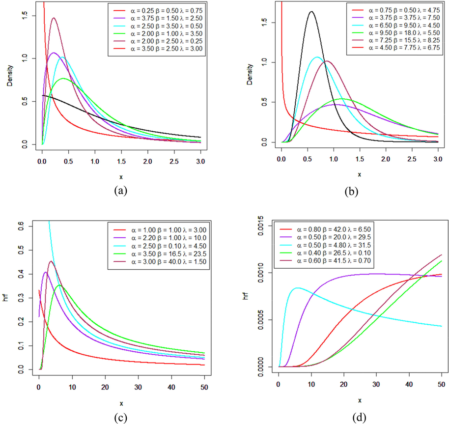
Density function 1 (a) and 1 (b) and hazard rate function 1 (c) and 1 (d) at different parameter values.
Table: Some special models of MOEIK distribution.
Special Cases
Resultant model
Pdf for
Lomax distribution
Marshall-Olkin Lomax
Beta type II
Marshall-Olkin Beta type II
The log-logistic (Fisk) distribution
Marshall-Olkin log-logistic
2.3 Quantile function
Let random variable
having pdf in Eq. (5). The computation of the quantile function, say
of the MOEIK distribution can be attained by inverting Eq. (6)
3 Properties of MOEIK distribution
This section provides unambiguous expressions for some major properties of the observed distribution starting from the ordinary moments.
3.1 Moments
This subsection provides the unambiguous expressions of the rth non-central moment and cumulants. Numerous important features and characteristics such as tendencies, coefficient of skewness, coefficient of kurtosis and dispersions can be studied from moments. The given theorem provide moments.
The rth raw moments of the MOEIK distribution can be obtained by following the definition of the moments as
The cumulants of the MOEIK distribution are attained from above expression as where . Thus,
The coefficient of skewness and the coefficient of kurtosis for the MOEIK distribution can also obtained from the third and the fourth standardized cumulants by using formulae
respectively. Table 1 represents the behavior of raw moments, skewness and kurtosis for MOEIK distribution.
Moments→
Skewness
Kurtosis
0.25
0.1567
0.0755
0.0985
0.3760
0.4097
65.961
0.75
0.2826
0.1896
0.2825
1.1204
0.7920
31.164
1.50
0.3974
0.3274
0.5398
2.2225
1.2115
20.731
2.50
0.5026
0.4808
0.8609
3.6718
1.6616
15.885
4.50
0.6478
0.7334
1.4549
6.5181
2.3928
12.118
7.50
0.7962
1.0410
2.2696
10.692
3.2844
9.8651
0.25
0.1643
0.1050
0.1564
0.6219
0.5890
56.385
0.75
0.3418
0.2746
0.4504
1.8523
1.1005
24.559
1.50
0.5026
0.4807
0.8609
3.6718
1.6616
15.886
2.50
0.6459
0.7087
1.3711
6.0602
2.2654
12.066
4.50
0.8370
1.0801
2.3096
10.741
3.2496
9.2058
7.50
1.0266
1.5265
3.5879
17.585
4.4521
7.5467
4.25
0.3281
0.3213
0.8082
9.3416
2.2608
90.457
4.75
0.2836
0.2267
0.4076
2.1659
1.1475
42.108
5.50
0.2356
0.1477
0.1859
0.5050
0.5427
23.146
6.50
0.1922
0.0935
0.0841
0.1374
0.2608
15.702
7.50
0.1623
0.0645
0.0451
0.0527
0.1486
12.661
9.50
0.1237
0.0360
0.0174
0.0129
0.0639
10.005
3.2 Incomplete moments
Researchers have general interest to compute the rth incomplete moments of life-time models. The incomplete moments are mostly utilized to explain the Bonferroni and Lorenz curves while it also helps to evaluate the mean deviation. Let X follows the MOEIK distribution and its rth incomplete moment could be evaluated from
3.3 Mean deviation
A most appropriate tool used to evaluate the average absolute deviation of the observation from their mean is mean deviation. We can find the mean deviation about the mean and median from the following expressions given respectively.
Mean deviation is used in numerous important fields such as economics, demography, insurance, medicines and reliability.
3.4 Mode
For symmetrical distributions such as the standard normal, t-distribution and Cauchy distribution, the mean, median and mode are same say 0. But for the asymmetrical distribution we have to follow the general method with necessary and sufficient conditions to find the mode. The mode of the MOEIK distribution can be obtained by taking the first derivative and equate it to zero.
.
The density function of the MOEIK in Eq. (6) is given as
Following the definition of mode
Since
. Therefore,
3.5 Rényi entropy
Entropy is generally belongs to statistical mechanics, more specifically microscopic variables. Therefore, more precisely we can say that Entropy is the measure of disorder in a microscopic system. A common measure of entropy is the Rényi entropy and has much importance in many fields such as statistical inference, classification, problems identification in statistics, econometrics and pattern recognition in computer sciences. The given theorem provides expression for Rényi entropy.
If the random variable X is defined as Eq. (6), then the Rényi entropy is given under the necessary condition that
If r.v X follows MOEIK distribution then Rényi entropy is defined as
After simplification, the expression becomes
Substitution completes the proof. □
3.6 Order statistics
Let the random variables and its ordered values are denoted as . The probability density function (pdf) of order statistics is obtained using the function
The density of the nth ordered statistics follows the MOEIK distribution is
The rth moment of order statistic is obtained as
On simplifications, we get
The expressions for rth moment of order statistic becomes
3.7 Maximum likelihood estimation
This study adopts the maximum likelihood estimation method so that it is mostly used and provides the maximum information about the properties of the estimated parameters. Moreover, the normal approximation of these estimators can frankly be managed systematically and mathematically for large sample theory. Consequently, the ML estimation has adopted to estimate the unknown parameters of the MOEIK distribution.
Let random variable X belong to the observed distribution and have vector of the parameters with size n. The sample likelihood function is achieved as
The log-likelihood function is
Now we have to maximize the log-likelihood function given in Eq. (20) to get the ML estimates of unknown parameters of the Marshall-Olkin extended Kumaraswamy distribution. For this purpose, we take the first derivative of the log-likelihood equation with respect to parameters and equate to zero respectively.
The exact solution of the derived ML estimator for unknown parameters in Eqs. (21)–(23) is genuinely not possible. Therefore, it is more appropriate to use the nonlinear optimization algorithms such as a Newton-Raphson algorithm for maximizing the likelihood function numerically. We can use R (optimal function or maxBFGS function), or MATHEMATICA (Maximize function). After application of large sample property of the ML Estimates, MLE
can be treated as being approximately normal with the mean θ and the variance-covariance matrix equal to the inverse of the expected information matrix, i.e.
is the information matrix then its inverse of matrix is
provide the variances and covariance’s. The
variance-covariance matrix is actually equal to the inverse of the expected information matrix
is given as
The elements of the variance-covariance information matrix are given in Appendix.
4 Simulation
To inspect the performance of the Marshall-Olkin extended inverted Kumaraswamy distribution, we conduct a simulation study by using the Monte Carlos simulation method with 10,000 repetitions on the basis of the bias and the mean square error of the estimated parameters from the maximum likelihood estimation method. The simulation is done as follows:
Data is generated from , where is uniformly distributed (0, 1).
are taken as the true parameter values .
Simulation is conducted for the sample sizes .
The repetition of the experiment is 10,000 times for each sample size.
Table 2 represents the outcomes of the Monte Carlos simulation study. We evaluate the mean of estimated parameters, mean square errors (MSE) and biases. These findings based on the expected first order asymptotic theory as the bias and the MSE’s decreases toward zero with the increase in sample size.
True parameters
Sample size
Parameters
Summaries of Parameters
Mean
Bias
MSE
1.25
2.50
0.75
10
1.625
0.375
111.6
2.828
0.328
1.330
0.777
0.027
0.026
50
1.305
0.055
0.085
2.556
0.056
0.162
0.755
0.005
0.004
100
1.276
0.026
0.036
2.532
0.032
0.078
0.753
0.003
0.002
200
1.262
0.012
0.017
2.515
0.015
0.037
0.751
0.001
0.001
2.5
3
1.5
10
6.065
3.565
709.1
3.264
0.264
1.131
1.556
0.056
0.108
50
2.665
0.165
0.601
3.047
0.047
0.157
1.510
0.010
0.016
100
2.582
0.082
0.236
3.025
0.025
0.079
1.505
0.005
0.008
200
2.536
0.036
0.098
3.013
0.013
0.038
1.503
0.003
0.004
The observations in Table 2 direct the MSE of the ML estimators of decreases and their biases decay towards 0 as sample size increases. While the increase in shape parameters, MSE of estimated parameters increases.
5 Applications
This section represents the potentiality and flexibility of the new model as compared to some other existing life-time models by using some real-life examples.
-
The first real-life data was originally reported by Hinkley (1977). Data consists of 30 observations of the March precipitation (in inches) in Minneapolis/St Paul. The observed values are
| 0.77 | 1.74 | 0.81 | 1.20 | 1.95 | 1.20 | 0.47 | 1.43 | 3.37 | 2.20 | 3.00 | 3.09 |
| 1.51 | 2.10 | 0.52 | 1.62 | 1.31 | 0.32 | 0.59 | 0.81 | 2.81 | 1.87 | 1.18 | 1.35 |
| 4.75 | 2.48 | 0.96 | 1.89 | 0.90 | 2.05 |
-
The second data also consists of 30 values for the failure time of repairable objects used by Murthy et al. (2004). The observed values are
| 1.43 | 0.11 | 0.71 | 0.77 | 2.63 | 1.49 | 3.46 | 2.46 | 0.59 | 0.74 | 1.23 | 0.94 |
| 4.36 | 0.40 | 1.74 | 4.73 | 2.23 | 0.45 | 0.70 | 1.06 | 1.46 | 0.30 | 1.82 | 2.37 |
| 0.63 | 1.23 | 1.24 | 1.97 | 1.86 | 1.17 |
-
The third application is initially used by Bhaumik et al. (2009). The observed values
| 5.1 | 1.2 | 1.3 | 0.6 | 0.5 | 2.4 | 0.5 | 1.1 | 8.0 | 0.8 | 0.4 | 0.6 |
| 0.9 | 0.4 | 2.0 | 0.5 | 5.3 | 3.2 | 2.7 | 2.9 | 2.5 | 2.3 | 1.0 | 0.2 |
| 0.1 | 0.1 | 1.8 | 0.9 | 2.0 | 4.0 | 6.8 | 1.2 | 0.4 | 0.2 |
| Min. | Q1 | Median | Q3 | Mean | Max. | |
|---|---|---|---|---|---|---|
| Data 1 | 0.320 | 0.915 | 1.470 | 2.088 | 1.675 | 4.750 |
| Data 2 | 0.110 | 0.717 | 1.235 | 1.943 | 1.543 | 4.730 |
| Data 3 | 0.100 | 0.500 | 1.150 | 2.475 | 1.879 | 8.000 |
By using these data sets, we have made comparison for the new generated Marshall-Olkin extended inverted Kumaraswamy (MOEIK) distribution with the Generalized Inverted Kumaraswamy (GIK), Transmuted Exponentiated Inverse Rayleigh (TEIR), Logistic Weibull (LW), Transmuted Power Lindley (TPL), Marshall Olkin Frechet (MOFr) and Inverted Kumaraswamy (IK) distribution. We use numerous goodness of fit measures to compare the new developed model with other existing models such as the log likelihood function (−2l), Akaike Information Criterion (AIC), Bayesian Information Criterion (BIC), Consistent Akaike Information Criterion (CAIC), Hanna-Quinn Information Criterion (HQIC), Kolmogrov-Smirnov (K-S), Anderson Darling (A∗) and Cramer-von Mises (W∗). The pdf of other existing models are stated below.
Generalized Inverted Kumaraswamy Distribution (Iqbal et al., 2017) where are shape parameters.
Transmuted Exponentiated Inverse Rayleigh Distribution (Haq, 2016) where is shape parameter, is scale parameter and is transmuted parameter.
Logistic Weibull Distribution (Tahir et al., 2016) where are shape parameters.
Transmuted Power Lindley Distribution (Granzotto et al., 2016) where
Marshall Olkin Fréchet Distribution (Krishna et al., 2013) where are positive shape parameters while is scale parameter.
Tables 4–6 provide the estimated parameters and goodness of fit measures of three real life data sets. It is obvious from the tables that the goodness of fit measures such as AIC, BIC, CAIC, HQIC, K-S, A∗ and W∗ of the new developed MOEIK distribution are less than that of the GIK, TEIR, LW and IK distribution, therefore, considered as a best fitted model. Figs. 2, 3 and 4 show the histogram of data with estimated pdf curves (left side) and also explain the estimated and the empirical cdf curves (right side). It is clear from the above tables and figures that the MOEIK distribution provides better fit as compared to other existing models. These bold values highlight the model which have better fit as compared to competitor models. These bold values highlight the model which have better fit as compared to competitor models. These bold values highlight the model which have better fit as compared to competitor models.
Models
Estimates (Std. Error)
−2l
AIC
BIC
CAIC
HQIC
K-S
A*
W*
4.3228 (0.9387)
6.5798 (5.0017)
6.9226 (9.6043)
76.69
82.69
86.89
84.79
84.03
0.068
0.137
0.019
1.9552 (1.8117)
3.9501 (5.6951)
1.4202 (1.0211)
78.63
84.63
88.84
86.77
85.98
0.110
0.318
0.052
6.5630 (80.152)
0.0958 (1.1693)
−0.6700 (0.2661)
84.20
90.20
94.41
92.30
91.55
0.182
1.139
0.212
2.7709 (243.47)
0.3635 (32.322)
1.0061 (88.405)
77.86
83.86
88.06
85.96
85.21
0.074
0.191
0.025
1.5965 (0.2054)
0.4801 (0.1643)
0.5812 (0.6548)
77.30
83.31
89.05
86.18
86.19
0.091
0.146
0.029
42.598 (2.8490)
2.6975 (0.4482)
0.3548 (0.2109)
77.60
83.60
87.80
85.70
84.94
0.095
0.224
0.024
2.9872 (0.4730)
8.5899 (3.1222)
–
78.85
83.85
87.65
85.25
84.74
0.114
0.338
0.055
Models
Estimates (Std. Error)
−2l
AIC
BIC
CAIC
HQIC
K-S
A*
W*
3.8031 (0.8166)
2.1861 (2.0393)
9.6185 (14.059)
79.60
85.60
89.80
87.70
86.94
0.078
0.119
0.017
1.1623 (1.0228)
1.4462 (1.3918)
1.8481 (1.1813)
81.64
87.64
91.84
89.74
88.98
0.109
0.284
0.048
7.2940 (25.055)
0.0254 (0.0871)
−0.8803 (0.1142)
117.0
123.0
127.2
125.1
124.3
0.376
1.366
1.471
2.8927 (293.52)
0.5531 (33.237)
0.7775 (78.895)
80.83
86.83
91.03
88.93
88.17
0.083
0.177
0.023
1.3380 (0.1743)
0.6301 (0.1927)
0.5356 (0.5587)
80.73
86.73
90.93
88.83
88.07
0.089
0.180
0.025
63.165 (6.7032)
2.1070 (0.3087)
0.1669 (0.0608)
81.53
87.53
91.73
89.63
88.87
0.104
0.283
0.043
2.4609 (0.4214)
4.1716 (1.2783)
–
82.48
86.48
90.28
88.88
87.37
0.111
0.340
0.052
Models
Estimates (Std. Error)
−2l
AIC
BIC
CAIC
HQIC
K-S
A*
W*
2.1193 (0.5717)
1.7026 (0.8020)
2.2471 (2.3570)
110.9
116.9
121.5
119.2
118.5
0.082
0.233
0.035
2.0236 (1.8839)
2.6369 (3.8684)
0.8858 (0.6642)
111.5
117.5
122.1
119.8
119.1
0.095
0.281
0.039
6.9784 (12.604)
0.0138 (0.0247)
−0.7798 (0.1350)
170.8
176.8
181.4
179.1
178.3
0.429
18.01
2.294
2.7709 (193.53)
0.7056 (17.189)
0.5526 (38.601)
111.9
117.9
122.5
120.2
119.5
0.085
6.327
0.633
0.9265 (0.1156)
0.7453 (0.2414)
0.4094 (0.5958)
111.2
117.2
122.5
120.5
119.7
0.091
0.280
0.048
29.053 (2.3853)
1.4730 (0.2397)
0.1124 (0.1098)
111.4
117.4
121.9
119.7
119.3
0.089
0.289
0.043
1.7409 (0.3238)
2.1058 (0.5373)
–
112.5
117.5
122.6
120.1
119.6
0.096
0.279
0.039
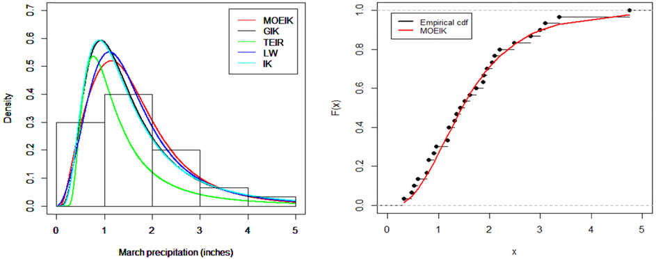
The fitted densities (left) and estimated cdf (right) on Data set 1.
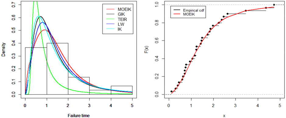
The fitted densities (left) and estimated cdf (right) on Data set 2.
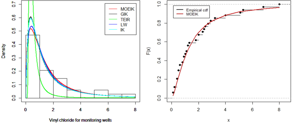
The fitted densities (left) and estimated cdf (right) on Data set 3.
6 Conclusion
The study reveals a generalization of the Inverted Kumaraswamy distribution and elaborates explicit expression for some of its major properties. The study also explains the behavior of the estimated parameters by using the Monte Carlos simulation approach. Three real-life applications have also presented for the demonstration of enhanced flexibility and better fit of the observed model as compared to the other considered existing models.
References
- Burr type III distribution: properties and estimation. Egypt. Stat. J.. 1999;43:102-116.
- [Google Scholar]
- Inverted Kumaraswamy distribution: properties and estimation. Pak. J. Stat.. 2017;33(1)
- [Google Scholar]
- Testing parameters of a gamma distribution for small samples. Technometrics. 2009;51(3):326-334.
- [Google Scholar]
- On the maximum likelihood and least-squares estimation in the Inverse Weibull distributions. Stat. Appl.. 1990;2(1):53-66.
- [Google Scholar]
- Inverted exponential distribution as a life distribution model from a Bayesian viewpoint. Data Sci. J.. 2007;6:107-113.
- [Google Scholar]
- Statistical inference for Kumaraswamy distribution based on generalized order statistics with applications. Br. J. Math. Comput. Sci.. 2014;4(12):1710.
- [Google Scholar]
- The inverse Gaussian distribution and its statistical application – a review. J. R. Stat. Soc. Ser. B (Methodological) 1978:263-289.
- [Google Scholar]
- Grain yield reliability analysis with crop water demand uncertainty. Stochastic Environ. Res. Risk Assess.. 2006;20(4):259-277.
- [Google Scholar]
- Statistical study of monthly rainfall trends by using the transmuted power Lindley distribution. Int. J. Stat. Prob.. 2016;6(1):111.
- [Google Scholar]
- Transmuted exponentiated inverse Rayleigh distribution. J. Stat. Appl. Prob.. 2016;5(2):337-343.
- [Google Scholar]
- The Marshall-Olkin length-biased exponential distribution and its applications. J. King Saud Univ. Sci. 2017 (Published online)
- [Google Scholar]
- Generalized Inverted Kumaraswamy distribution: properties and application. Open J. Stat.. 2017;7(04):645.
- [Google Scholar]
- Kumaraswamy’s distribution: a beta-type distribution with some tractability advantages. Stat. Methodol.. 2009;6(1):70-81.
- [Google Scholar]
- Applications of Marshall-Olkin Fréchet distribution. Commun. Stat. Simul. Comput.. 2013;42(1):76-89.
- [Google Scholar]
- A generalized probability density function for double-bounded random processes. J. Hydrol.. 1980;46(1–2):79-88.
- [Google Scholar]
- The exponentiated Kumaraswamy distribution and its log-transform. Braz. J. Prob. Stat.. 2013;27(1):31-53.
- [Google Scholar]
- A new method for adding a parameter to a family of distributions with application to the exponential and Weibull families. Biometrika. 1997;84(3):641-652.
- [Google Scholar]
- Weibull Models. Vol vol. 505. John Wiley & Sons; 2004.
- Acceptance sampling based on the inverse Rayleigh distribution. Econ. Qual. Control. 2005;20(2):277-286.
- [Google Scholar]
- Maximization of manufacturing yield of systems with arbitrary distributions of component values. Ann. Oper. Res.. 2000;99(1):373-383.
- [Google Scholar]
- The inverse Lindley distribution: a stress-strength reliability model with application to head and neck cancer data. J. Ind. Prod. Eng.. 2015;32(3):162-173.
- [Google Scholar]
- Bayesian analysis of the Kumaraswamy distribution under failure censoring sampling scheme. Int. J. Adv. Sci. Technol.. 2013;51:39-58.
- [Google Scholar]
- The Logistic-X family of distributions and its applications. Commun. Stat. Theory Methods. 2016;45(24):7326-7349.
- [Google Scholar]
- On the inverse Rayleigh distributed random variable. Rep. Stat. Appl. Res. JUSE. 1972;19:13-21.
- [Google Scholar]
Appendix


