

Translate this page into:
The improved preconditioned iterative integration-exponential method for linear ill-conditioned problems
*Corresponding author E-mail address: jlcheng@cumtb.edu.cn (J. Cheng).
-
Received: ,
Accepted: ,
Abstract
The preconditioned iterative integration-exponential method is an innovative iterative regularization technique designed to solve ill-conditioned linear problems. However, the preconditioned iterative integration-exponential method has been primarily applied to symmetric positive definite problems, and a notable limitation is its inability to adaptively determine the optimal number of iterations. To overcome this limitation, the present study demonstrates that the preconditioned iterative integration-exponential method can also be effectively applied to nonsymmetric positive definite linear systems. Furthermore, an improved preconditioned iterative integration-exponential method is proposed by combining the iterative refinement algorithm with the original approach. Addressing the challenge of adaptively determining the optimal number of iterations and Krylov subspace can solve the problem of low computational efficiency of the improved preconditioned iterative integration-exponential method in dealing with large-scale and sparse problems. Numerical results show that the newly proposed method is more robust than the original one.
Keywords
First order dynamical systems
Ill-conditioned problems
Iterative integration-exponential
Precise integration method

1. Introduction
In recent years, ill-conditioned problems have attracted more and more attention and have been widely used in engineering and mathematics fields, such as geodesy (Yu et al., 2023), geophysical exploration (Li et al., 2024), and signal and processing (Wu, 2012; Yang and Deng, 2017). The solution methods of ill-conditioned equations have research significance.
The ill-conditioned system can be expressed as:
where is an ill-conditioned matrix, is the solution, and is the observation. For an ill-conditioned system, a small disturbance in or can result in a significantly larger change in the solution This phenomenon presents considerable challenges when attempting to solve the system (1) numerically. Consequently, the application of conventional numerical methods for solving such systems (1) may prove ineffective. To address this issue, several iterative regularization methods have been developed and widely used, including Tikhonov regularization (Benning and Burger, 2018; Chang et al., 2024; W. Wang et al., 2024) (TR), Landweber iteration (Mittal and Giri, 2021), and direct regularization methods like truncated singular value decomposition (Xu et al., 2024; Xu, 1998) (TSVD), truncated generalized singular value decomposition (Chen and Chan, 2017), and truncated randomized singular value decomposition (Bai et al., 2021; Huang et al., 2022). A notable characteristic of these regularization methods is that their performance depends on various regularization parameters, such as the truncation order in TSVD, the Tikhonov regularization parameter, and the number of iterations in iterative regularization methods. In recent years, iterative regularization methods for ill-conditioned equations that are based on the numerical solutions of dynamic systems have garnered attention (Dmytryshyn et al., 2022; Edvardsson et al., 2015).
The exploration of the connections between iterative numerical methods and continuous dynamical systems often deepens the understanding of iterative numerical techniques. Additionally, this investigation aids in the advancement of enhanced iterative numerical methods by utilizing numerical approaches for ordinary differential equations and continuous dynamical systems (Chu, 1988; Miyatake et al., 2018). For solving ill-conditioned linear systems, Ramm (2004) developed the dynamical systems method. Wu (2002) analyzed the relationship between Wilkinson iteration method and Euler method and proposed a new iterative improved solution method to solve the problem of ill-conditioned linear equations. Enlightened by Wu’s work, Salkuyeh et al. (2011) proposed a new two-step iterative method. Beik et al. (2018) presented a generalized two-step iterative method. For symmetric positive definite linear ill-conditioned systems, Hoang and Ramm (2010) proposed a gradient algorithm for dynamic systems based on SVD decomposition, Wu (2023) introduced an exponential approximation method.
The precise integration method, proposed by Zhong (2004), is designed to calculate the matrix exponential. It is known for its high efficiency and precision, often yielding results nearly equivalent to exact solutions on a computer. As a result, it is widely used in solving various dynamic systems (J. Wang et al., 2024; Yang et al., 2021; Zhu et al., 2023, 2021). Fu and Zhang (2011) introduced a precise integration method for solving positive definite ill-conditioned linear systems and proposed an iterative integration-exponential (IIE) method. Huang et al. (2021) gave rigorous proof of the convergence of the IIE method and discovered that: (1) the IIE method is an iterative regularization method similar to the TR method; (2) the Landweber iterative algorithm can be seen as a special form of the IIE method; (3) The number of iterations can be equivalent to the regularization parameter of the IIE method. In order to improve the precision of calculation and reduce the number of iterations, a preconditioned IIE (PIIE) method (Fu and Li, 2018) was proposed. The PIIE method has demonstrated effective results in addressing ill-conditioned systems, particularly in geoscience (Kailiang et al., 2023). However, determining the optimal number of iterations is an area requiring further research.
To solve this problem, this paper proposes an improved preconditioned precise integration iterative (IPIIE) method. The new method uses the residual error to correct the error of the solution of the original PIIE method, which avoids the selection of the optimal iteration termination parameter.
2. A brief review of the PIIE method
2.1 The IIE method
Multiply the transpose of the matrix on both sides of Eq. (1).
Consider the following linear dynamical systems
Hoang and Ramm (2010) transformed solving linear eqs. (2) into solving linear dynamical system (3). The solution of a linear dynamical system (3) can be expressed as
Here, the is a symmetric positive definite matrix. When approaches infinity and is zero vector, can be expressed as
where Let be small enough and set
then the can be written in the following iterative form:
To take this further, set
and by combining Eqs. (7) and (8), an iterative formula can be derived as follows.
In the IIE method, the matrix exponential in Eq. (9) is computed through precise integration. By Taylor expansion, it is obtained that
here, denotes the truncation order of Taylor expansion, and denotes the identity matrix. Consequently, in Eq. (7) can be calculated using the following formula:
where is the approximate value of . By combining Eq. (5), (7) and (12), the IIE method for solving linear equations can be expressed in the following form:
where the initial value is . For IIE method, the iteration number k is considered as the regularization parameter.
2.2 The PIIE method and termination iteration condition
In order to accelerate the convergence speed of IIE, the PIIE method uses 1-norm normalization to reduce the condition number of the coefficient matrix.
Multiplying the preconditioned matrix on both sides of the Eq. (2)
The definition of the matrix is as follows:
where is the element of the matrix .
Fu et al. (2018) proposed an iterative termination condition for the PIIE algorithm. The error of the iteration is defined as
and define the following function:
The parameter is an integer. When , the iteration ends.
| Algorithm 1: The PIIE algorithm |
|---|
|
1: Compute the preconditioned matrix , . 2: Compute and . 3: Compute the initial value 4: while satisfying termination conditions; 5: 6: 7: end |
2.3 The PIIE method for nonsymmetric positive definite linear system
The PIIE method is suitable for symmetric positive definite matrix linear systems (Huang et al., 2021). In this section, we extend the proof to demonstrate that the PIIE method is also applicable to solving nonsymmetric positive definite linear systems. Consider the following linear system
where is a nonsymmetric positive real definite matrix.
Theorem 1. Let be a nonsymmetric positive definite matrix, be a positive real number
we have
The following two lemmas are used to prove Theorem 1.
Lemma 1. Let be a nonsymmetric positive definite matrix, be a positive real number
Proof: According to the definition of matrix exponential, can be written as:
it is easy to find .
Lemma 2. Let be a nonsymmetric positive definite matrix, be a positive real number
where is zero matrix.
Proof: Consider the following linear dynamic systems of equations
where is an arbitrarily preassigned vector, and is a positive definite matrix. The exact solution of a dynamic system (24) can be expressed as:
The proof investigates two aspects regarding the existence of both repeated and non-repeated eigenvalues within the matrix.
-
(1)
Assume has different eigenvalues and is the eigenvector corresponding to the eigenvalue.
The solution (Boyce and DiPrima, 1986) of linear dynamic system (24) can also be written as follows
(26)where is a constant, determined by the initial value . Because is a positive definite matrix, the eigenvalues of are less than 0. When approaches infinity, we can have .
-
(32)
Assume the has different eigenvalues , are the eigenvector corresponding to the eigenvalues, where .
It means that there are repeated eigenvalues. In this case, the number of corresponding linearly independent eigenvectors is smaller than the algebraic multiplicity of the eigenvalue. Assume the maximum algebraic multiplicity to be . The solution (Boyce and DiPrima, 1986) of a linear dynamic system (24) can be written as follows
(27)Where is a polynomial matrix, its degree is no more than . Because is a positive definite matrix, the eigenvalues of are less than 0. When approaches infinity, it is easy to get , so .
Based on the discussion above, we can get
Since is an arbitrarily preassigned vector, we can get .
According to Lemma 1, we can get
Let , then
According to Lemma 2, we can get
The PIIE method is appropriate for asymmetric positive definite linear systems, as demonstrated by the aforementioned proof.
3. The IPIIE method
The termination iteration condition proposed by Fu et al. (2018) facilitates the selection of the optimal number of termination iterations for the PIIE method. The optimal iteration termination parameter can be regarded as an alternative form of the PIIE regularization parameter. This section initially demonstrates, through a straightforward example, that for a given coefficient matrix, the observed values have a significant impact on the optimal termination iteration parameter. To enhance the computational accuracy of the PIIE method and to enable adaptive selection of parameters for iteration termination, this section introduces an improved algorithm that integrates the PIIE with the Iterative Refinement Method. This innovative combination of algorithms significantly enhances both the accuracy and robustness of the PIIE method.
3.1 The optimal termination iteration parameters
Considering the typical ill-conditioned linear nonsymmetric positive definite system with Hilbert matrices , where
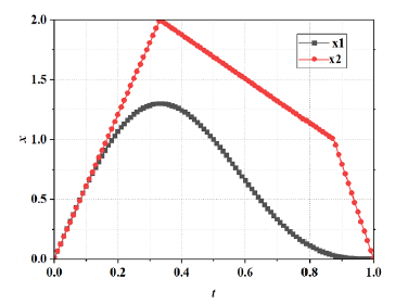
In this experiment, m is 300, the condition number of is 3.93e+19. Assume that the two exact solutions of the Eq. (32) are
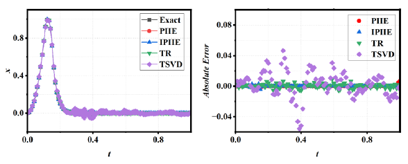
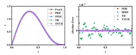
with . And the two observations are and . Fig. 1 illustrates that when the iteration termination parameter n is set to 2, the PIIE method yields satisfactory results with, . However, when the termination parameter is unchanged, a noticeable deviation arises between the PIIE method’s results and the exact solution with . Fig. 2 further demonstrates that as the parameter n increases, the solution from the PIIE method gradually converges to the exact solution, achieving satisfactory results when .
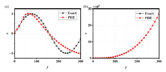
- The numerical results of the PIIE method. The termination iteration parameter n is 2. (a)
(b)
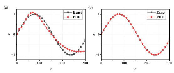
- The numerical results of the PIIE method with
. The parameter of the termination iteration parameter n takes different values (a) n=4 (b) n=5.
This numerical experiment demonstrates that, for a given coefficient matrix, the observed value has a substantial impact on the optimal termination iteration parameter, denoted as n.
3.2 The theory IPIIE method
Iterative refinement is a significant numerical technique used to improve the accuracy of initial solutions in various computational problems, especially in the context of solving linear systems and conducting numerical computations (Cui et al., 2023; Pan et al., 2021). The core principle of iterative refinement involves starting with an approximate solution and iteratively adjusting it based on the residuals or errors observed from the initial solution.
Let A and be as in Eq. (18). Then, the iterative refinement algorithm defines the solution to Eq. (18) iteratively by,
with as initial model. The solution of Eq. (34) is , then
This iterative process continues until a desired level of accuracy or convergence is achieved, thereby improving the overall precision of the solution obtained.
Inspired by the Iterative Refinement method, the integration of this method with the PIIE algorithm can enhance the accuracy of numerical solutions. The steps for the calculation are outlined as follows:
-
(1)
The Algorithm 1 is used to calculate the initial value, and the iteration termination parameter n is 2.
-
(2)
Calculation of the residual vector :
(36) -
(3)
If the residual satisfies the threshold, stop the calculation. Otherwise, use the PIIE approach to solve the Eq. (37):
(37) -
(4)
Correcting the calculation results:
(38)
Repeat steps 2 to 4 until the residual is sufficiently small or a predetermined number of iterations is reached.
| Algorithm 2: The IPIIE algorithm |
|---|
|
1: Compute the preconditioned matrix , . 2: 3: Compute 4: while until satisfy termination conditions. 5: 6: 7: end |
3.3 Convergence analysis
The Algorithm 2 is a combination algorithm. As long as the PIIE convergence is guaranteed, IPIIE can be guaranteed to be convergent. Huang et al. (2021) studied the above problems in detail.
The PIIE method uses row normalization to preprocess the matrix. According to the Gershgorin Circle Theorem (Bell, 1965), the in Eq. (14) is less than or equal to 1.
If , , with defined in Eqs. (10) and denote the spectral radius of a matrix. For the PIIE method
When k tends to infinity, PIIE will converge with .
3.4 The validation of the IPIIE algorithm
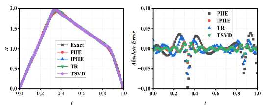
This section still uses the Hilbert matrix model in subsection 3.1 to test the robustness of the IPIIE algorithm. Assume that the exact solution of the Eq.(32) are
with .The value of is the same as that of the in subsection 3.1. The relative error (RE) is
where is numerical solution and is a true solution.
According to subsection 3.1 the optimal termination iteration parameter is 5. The relative error of PIIE algorithm is 1.26e-2, and the relative error of IPIIE is 2.06e-3. According to Fig. 3 and the relative error of the two algorithms, it can be concluded that the IPIIE algorithm is better than that of the optimal solution of the PIIE algorithm.
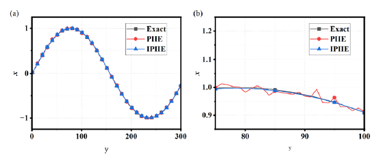
- The numerical results of the PIIE and IPIIE methods with
. The parameter of the termination iteration parameter n of PIIE is 5. (a) Original drawing and (b) Drawings of partial enlargement.
Numerical tests indicate that the IPIIE method consistently outperforms the PIIE method. IPIIE delivers accurate results without requiring adjustments to the termination iteration parameter n, effectively reducing the sensitivity of termination iteration parameters to observations compared to PIIE.
4. Numerical experiments
All numerical experiments in this subsection were carried out using MATLAB R2024b on a laptop computer with an Intel Core i7-12700H CPU and 64 GB of RAM.
4.1 Ill-conditioned problems in one space-dimension
Considering the test problems (Hansen, 2007) heat and gravity , are linear discrete ill-posed problems. These examples originate from the discretization of Fredholm integral equations of the first kind, which have the general form:
where is observable, is a known kernel function. The Eq. (43) is transformed into Eq. (44) by discretizing into N points,
where is matrix, usually an ill-conditioned matrix.
Examples 1
In this example,
where . The three desired solutions are shown in Fig. 4. In this example, N is 1000, and the condition number of is 2.33e+232.
- The desired solution.ti
When , the optimal regularization parameter for the TR method is 1e-10, the optimal number of truncated singular values for the TSVD method is 813, and the optimal termination iteration parameter for the PIIE method is 4. The relative errors for the numerical results of PIIE, IPIIE, TR, and TSVD are 3.10e-03,2.95e-03, 3.62e-03, and 7.10e-02, respectively. Fig. 5 demonstrates close agreement between the results of PIIE, IPIIE, and TR, while the TSVD method exhibited substantially larger errors in detail.
- The numerical results and absolute errors of the PIIE, IPIIE, TR and TSVD methods.
Examples 2
In geological exploration, the location, shape, and some parameters of geological anomalies occurring in the interior of the earth are usually determined according to the data measured on the surface of the earth. Assuming that the vertical component of the gravity field is measured on the surface, the mass distribution is located at depth . This inverse problem can be expressed as the Fredholm integral equation of the first kind, and its kernel function is
where , and is 0.5. The two desired solutions and are shown in Fig. 6
- The two desired solutions
.
When , the optimal regularization parameter for the TR method is 1e-11, the optimal number of truncated singular values for the TSVD method are 22, and the optimal termination iteration parameter for the PIIE method is 2. Fig. 7 illustrates that all four methods yield satisfactory computational results. However, the relative errors for the numerical results of PIIE, IPIIE, TR, and TSVD are 1.23e-06,1.22e-06, 3.24e-04 and 1.62e-06, respectively. From these results, it is evident that the computational accuracy of PIIE, IPIIE, and TSVD is comparable, while the TR method exhibits the lowest accuracy.
- When
, the numerical results and absolute errors of the PIIE, IPIIE, TR and TSVD methods.
When , the optimal regularization parameter for the TR method is determined to be 1e-12, while the optimal number of truncated singular values for the TSVD method is identified as 24. In addition, the optimal termination iteration parameter of the PIIE method is 3. Fig. 8 shows that there is a certain deviation between the numerical results of the four methods and the exact solution. However, the relative errors associated with the numerical results of PIIE, IPIIE, TR, and TSVD are 1.93e-02, 4.93e-03,1.13e-02, and 6.21e-03, respectively. These findings indicate that the computational accuracy of IPIIE and TSVD is comparable, whereas TR and PIIE exhibit the lowest levels of accuracy.
- When
, the numerical results and absolute errors of the PIIE, IPIIE, TR and TSVD methods.
4.2 Ill-conditioned problems in two space-dimensions
The test problem blurs that it is a linear discrete ill-posed problem. The blurring of the image is caused by a blurring function with parameters and . This blurring function can be determined using the regularization tool package (Hansen, 2007). In this example, the image size is , as shown in Fig. 9. The PIIE, TR and TSVD methods are compared. The optimal regularization parameter for the TR method has been determined to be 1e-12, while the optimal number of truncated singular values for the TSVD method is identified as 1441. Furthermore, the optimal termination iteration parameter for the PIIE method is established as 3. The numerical results are shown in Fig. 10. The relative errors associated with the numerical results of the PIIE, IPIIE, TR, and TSVD methods are 3.98e-01, 5.07e-02, 5.11e-02, and 1.55e-01, respectively. These findings suggest that the computational accuracy of the IPIIE and TR methods is comparable, whereas the TSVD and PIIE methods demonstrate the lowest levels of accuracy.
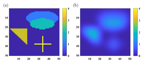
- (a) Original test image, (b) The deblurred image.
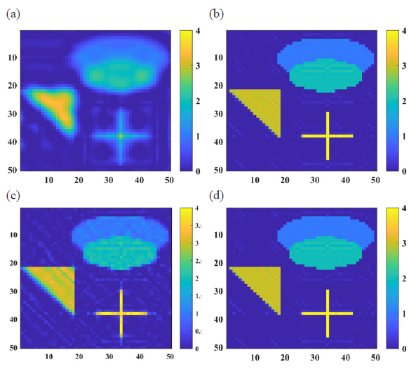
- The calculation results of different methods. (a) PIIE, (b) TR, (c) TSVD and (d) IPIIE.
In summary, compared with the PIIE, TR, and TSVD methods, the IPIIE method does not require the selection of optimal normalization parameters. Furthermore, the IPIIE method demonstrates enhanced applicability in addressing complex problems.
5. Discussion
The PIIE and IPIIE algorithms use precise integration to calculate the matrix exponential in Eq. (9). in the Eq. (13) results in high computational complexity. If is the sparse matrix, it can quickly densify the matrix during iteration, significantly increasing computational complexity and memory requirements. Consequently, when addressing large-scale, sparse, and ill-posed problems, the memory requirements for the PIIE and IPIIE methods increase significantly with a greater number of iterations. Fortunately, in the field of numerical solutions for differential equations, researchers have addressed similar limitations by proposing an exponential matrix calculation method that utilizes Krylov subspace techniques (Bergamaschi and Vianello, 2000; Botchev and Knizhnerman, 2020; Druskin and Simoncini, 2011; Fung and Chen, 2006; Suman and Kumar, 2022).
The Krylov subspace method transforms the original matrix exponential-vector product, as presented in the Eq. (9), into an m-dimensional matrix-vector product. The construction of the Krylov subspace basis through the Arnoldi process necessitates only matrix-vector product calculations. Furthermore, the dimension of the Krylov subspace is generally much smaller than the scale of the original problem. Consequently, this method can substantially decrease both computational complexity and memory requirements. For clarity, the PIIE and IPIIE based on the Krylov subspace are referred to as PIIE-K and IPIIE-K, respectively.
Considering the typical simple positive definite system with tridiagonal matrix .
In this case, m is 5000. Assume that the exact solution of the Eq. (32) are
with .
It can be seen from Fig. 11 that the number of non-zero elements in matrices and is 44,980 and 657,444, respectively. The memory consumption of matrices and in MATLAB is 1.258 MB and 178.100 MB, respectively. After 10 iterations, the number of non-zero elements in matrix increases by approximately 146 times, while the memory usage increases by approximately 141 times.
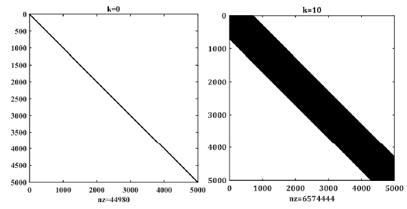
- A visual illustration of the number of non-zero elements in , the superscript k denotes the number of iterations.
is the number of non-zero elements, k is iteration times.
As illustrated in Table 1, when the termination iteration parameter n is set to 2, the computational time for the IPIIE method is significantly greater than that of the IPIIR-K method. Specifically, for m = 2000, the computation time for IPIIE is approximately 30 times longer than that of IPIIR-K, whereas for m = 5000, the computation time for IPIIE is about 12 times that of IPIIR-K. In terms of computational accuracy, at m = 2000, the relative errors for the PIIE and PIIE-K methods are 0.200 and 0.01126, respectively, while the relative errors for the IPIIE and IPIIE-K methods are 4.298e-07 and 2.319e-07, respectively. For m = 5000, the relative errors for the PIIE and PIIE-K methods remain at 0.200 and 0.01126, while the relative errors for the IPIIE and IPIIE-K methods are 4.012e-07 and 1.728e-07, respectively.
| Method | m=2000 | m=5000 | ||
|---|---|---|---|---|
| RE | Time | RE | Time | |
| PIIE(n=2) | 2.000e-01 | 7.223s | 2.000e-01 | 14.041s |
| PIIE-K(n=2) | 1.126e-02 | 0.057s | 1.126e-02 | 0.304 s |
| IPIIE | 4.298e-07 | 9.184s | 4.012e-07 | 20.520s |
| IPIIE-K | 2.319e-07 | 0.303s | 1.728e-07 | 1.683s |
6. Conclusions
This paper presents the IPIIE algorithms, which combine the iterative refinement method with the PIIE algorithms. Based on numerical experiments, the following conclusions have been drawn:
The PIIE is not only applicable to symmetric positive definite linear systems but also to asymmetric positive definite linear systems.
The IPIIE algorithm effectively alleviates the influence of observations on the optimal termination iteration parameters in the PIIE algorithm. An advantage of IPIIE is its avoidance of the need for selecting regularization parameters compared with TR and TSVD method.
The IPIIE-K method effectively reduces the high complexity and large memory consumption inherent in the PIIE method when solving large-scale, sparse problems, demonstrating significant advantages.
Additionally, the second-order dynamic system method for solving linear equations is ultimately reduced to solving a first-order dynamic system. Therefore, the application of the IPIIE algorithm within the second-order dynamic system method is further examined and discussed.
Acknowledgement
We would like to express our gratitude to the three anonymous reviewers for their thorough evaluation of our papers, as well as for their constructive feedback and valuable suggestions regarding the manuscripts.
CRediT authorship contribution statement
Jingtao Sun: Conceptualization, Methodology, Investigation, Writing – original draft, Software; Jiulong Cheng: Supervision, Writing – review & editing; Lei Qin: Resources, Writing – review & editing.
Declaration of competing interest
We declare that this research was conducted in the absence of any commercial or financial relationship that could be construed as a potential conflict of interest.
Declaration of Generative AI and AI-assisted technologies in the writing process
The authors confirm that there was no use of artificial intelligence (AI)-assisted technology for assisting in the writing or editing of the manuscript and no images were manipulated using AI.
References
- A novel modified TRSVD method for large-scale linear discrete ill-posed problems. Appl. Math. Sci.. 2021;164:72-88. https://doi.org/10.1016/j.apnum.2020.08.019
- [CrossRef] [Google Scholar]
- On the iterative refinement of the solution of ill-conditioned linear system of equations. Int. J. Comput. Math.. 2018;95:427-443. https://doi.org/10.1080/00207160.2017.1290436
- [CrossRef] [Google Scholar]
- Gershgorin’s theorem and the zeros of polynomials. Am. Math. Mon.. 1965;72:292. https://doi.org/10.2307/2313703
- [Google Scholar]
- Modern regularization methods for inverse problems. Acta Numerica. 2018;27:1-111. https://doi.org/10.1017/s0962492918000016
- [CrossRef] [Google Scholar]
- Efficient computation of the exponential operator for large, sparse, symmetric matrices. Numer. Linear Algebra Appl.. 2000;7:27-45. https://doi.org/10.1002/(sici)1099-1506(200001/02)7:1<27::aid-nla185>3.0.co;2-4
- [CrossRef] [Google Scholar]
- ART: Adaptive residual-time restarting for krylov subspace matrix exponential evaluations. J. Comput. Appl. Math.. 2020;364:112311. https://doi.org/10.1016/j.cam.2019.06.027
- [CrossRef] [Google Scholar]
- Elementary differential equations and boundary value problems - Fourth edition. 1986.
- A relaxed iterated tikhonov regularization for linear ill-posed inverse problems. J. Math. Anal. Appl.. 2024;530:127754. https://doi.org/10.1016/j.jmaa.2023.127754
- [Google Scholar]
- A truncated generalized singular value decomposition algorithm for moving force identification with ill-posed problems. J. Sound Vib.. 2017;401:297-310. https://doi.org/10.1016/j.jsv.2017.05.004
- [CrossRef] [Google Scholar]
- On the continuous realization of iterative processes. SIAM Rev.. 1988;30:375-387. https://doi.org/10.1137/1030090
- [CrossRef] [Google Scholar]
- Iterative refinement method by higher-order singular value decomposition for solving multi-linear systems. Appl. Math. Lett.. 2023;146:108819. https://doi.org/10.1016/j.aml.2023.108819
- [CrossRef] [Google Scholar]
- The dynamical functional particle method for multi-term linear matrix equations. Appl. Math. Comput.. 2022;435:127458. https://doi.org/10.1016/j.amc.2022.127458
- [CrossRef] [Google Scholar]
- Adaptive rational krylov subspaces for large-scale dynamical systems. Sys. Control Letters. 2011;60:546-560. https://doi.org/10.1016/j.sysconle.2011.04.013
- [CrossRef] [Google Scholar]
- Solvings through particle dynamics. Comput. Phys. Commun.. 2015;197:169-181. https://doi.org/10.1016/j.cpc.2015.08.028
- [Google Scholar]
- A Preconditioned precise integration method for solving Ill-conditioned linear equations. Appl. Math. Mech. (Engl. Ed.). 2018;39 https://doi.org/10.21656/1000-0887.380206
- [Google Scholar]
- A precise form for solving ill-conditioned algebraic equations and its iteration stopping criterion. Chin. J. Appl. Mech.. 2018;35 https://doi.org/10.11776/cjam.35.02.D008
- [Google Scholar]
- Precise integration method for solving il l-conditioned algebraic equations. Chin. J. Comput. Mech.. 2011;28 https://doi.org/10.7511/jslx(2011)04007
- [Google Scholar]
- Krylov precise time-step integration method. Numerical Meth Engineering. 2006;68:1115-1136. https://doi.org/10.1002/nme.1737
- [Google Scholar]
- Regularization tools version 4.0 for matlab 7.3. Numer. Algor.. 2007;46:189-194. https://doi.org/10.1007/s11075-007-9136-9
- [CrossRef] [Google Scholar]
- Dynamical systems gradient method for solving ill-Conditioned linear algebraic systems. Acta Appl. Math.. 2010;111:189-204. https://doi.org/10.1007/s10440-009-9540-3
- [CrossRef] [Google Scholar]
- A novel iterative integration regularization method for ill-posed inverse problems. Eng. Comput. 2020
- [Google Scholar]
- Tikhonov regularization with MTRSVD method for solving large-scale discrete ill-posed problems. J. Comput. Appl. Math.. 2022;405:113969. https://doi.org/10.1016/j.cam.2021.113969
- [CrossRef] [Google Scholar]
- Development of multi resolution transient electromagnetic virtual wave-field migration imaging method. J. Appl. Geophys.. 2024;222:105314. https://doi.org/10.1016/j.jappgeo.2024.105314
- [CrossRef] [Google Scholar]
- Transient electromagnetic pseudo wavefield imaging based on the sweep-time preconditioned precise integration algorithm. J. Appl. Geophys.. 2023;209:104937. https://doi.org/10.1016/j.jappgeo.2023.104937
- [Google Scholar]
- Iteratively regularized landweber iteration method: Convergence analysis via hölder stability. Appl. Math. Comput.. 2021;392:125744. https://doi.org/10.1016/j.amc.2020.125744
- [Google Scholar]
- On the equivalence between SOR-type methods for linear systems and the discrete gradient methods for gradient systems. J. Comput. Appl. Math.. 2018;342:58-69. https://doi.org/10.1016/j.cam.2018.04.013
- [CrossRef] [Google Scholar]
- Iterative refinement algorithm for efficient velocities and accelerations solutions in closed-loop multibody dynamics. Mech. Syst. Signal Process.. 2021;152:107463. https://doi.org/10.1016/j.ymssp.2020.107463
- [CrossRef] [Google Scholar]
- Dynamical systems method for solving operator equations. Commun. Nonlinear Sci. Numer. Simul.. 2004;9:383-402. https://doi.org/10.1016/s1007-5704(03)00006-6
- [CrossRef] [Google Scholar]
- A new iterative refinement of the solution of ill-conditioned linear system of equations. Int. J. Comput. Math.. 2011;88:950-956. https://doi.org/10.1080/00207161003713907
- [CrossRef] [Google Scholar]
- Investigation and implementation of model order reduction technique for large scale dynamical systems. Arch. Computat. Methods Eng.. 2022;29:3087-3108. https://doi.org/10.1007/s11831-021-09690-8
- [CrossRef] [Google Scholar]
- A memory-Efficient PITD method for multiscale electromagnetic simulations. IEEE Microw. Wireless Tech. Lett.. 2024;34:967-970. https://doi.org/10.1109/lmwt.2024.3408457
- [CrossRef] [Google Scholar]
- Tikhonov regularization with conjugate gradient least squares method for large-scale discrete ill-posed problem in image restoration. Appl. Math. Sci.. 2024;204:147-161. https://doi.org/10.1016/j.apnum.2024.06.010
- [CrossRef] [Google Scholar]
- An exponential approach to highly ill-conditioned linear systems. Appl. Math. Lett.. 2023;140:108560. https://doi.org/10.1016/j.aml.2022.108560
- [CrossRef] [Google Scholar]
- New iterative improvement of a solution for an ill-conditioned system of linear equations based on a linear dynamic system. Comput. Math. Appl. A. 2002;44:1109-1116. https://doi.org/10.1016/s0898-1221(02)00219-5
- [CrossRef] [Google Scholar]
- Parametric inverse of severely ill-conditioned hermitian matrices in signal processing. J. Franklin Institute. 2012;349:1048-1060. https://doi.org/10.1016/j.jfranklin.2011.12.006
- [CrossRef] [Google Scholar]
- Shape function method based on truncated singular value decomposition regularization for hull longitudinal bending moment identification. Measurement. 2024;232:114703. https://doi.org/10.1016/j.measurement.2024.114703
- [CrossRef] [Google Scholar]
- Truncated SVD methods for discrete linear ill-posed problems. Geophys. J. Int.. 1998;135:505-514. https://doi.org/10.1046/j.1365-246x.1998.00652.x
- [CrossRef] [Google Scholar]
- A dual interpolation precise integration boundary face method to solve two-dimensional transient heat conduction problems. Eng. Anal. Bound. Elem.. 2021;122:75-84. https://doi.org/10.1016/j.enganabound.2020.09.014
- [CrossRef] [Google Scholar]
- A data assimilation process for linear ill-posed problems. Math Methods App. Sci.. 2017;40:5831-5840. https://doi.org/10.1002/mma.4432
- [Google Scholar]
- An iterative and shrinking generalized ridge regression for ill-conditioned geodetic observation equations. J. Geod.. 2024;98 https://doi.org/10.1007/s00190-023-01795-1
- [CrossRef] [Google Scholar]
- On precise integration method. J. Computational Applied Math. 2004;163:59-78. https://doi.org/10.1016/j.cam.2003.08.053
- [CrossRef] [Google Scholar]
- An adaptively filtered precise integration method considering perturbation for stochastic dynamics problems. Acta Mech. Solida Sin.. 2023;36:317-326. https://doi.org/10.1007/s10338-023-00381-4
- [CrossRef] [Google Scholar]
- Low-Memory implementation of PITD method using a thresholding scheme. IEEE Microw. Wireless Compon. Lett.. 2021;31:537-540. https://doi.org/10.1109/lmwc.2021.3069643
- [CrossRef] [Google Scholar]


