The hazard rate function of the logistic Birnbaum-Saunders distribution: Behavior, associated inference, and application

1 Introduction

The failure rate function, also known as the hazard function (HF), is one approach to model life distributions in reliability and survival studies. Typically, researchers assume the hazard function (HF) of interest is either constant or monotonic. However, in practice, HFs may have a non-monotonic behavior, including, but are not limited to, upside-down bathtub-shaped HFs. Such functions increase to a point on the real line and then decrease to become constant later. Langlands et al. (1979) observed this HF in their study, which was about recovering from breast cancer. The study indicated that the highest mortality rate due to this type of cancer appears approximately three years after the disease was diagnosed; afterward, the mortality decreases slowly over a fixed time interval. In literature, three well-known continuous probability distributions have similar upside-down bathtub-shaped HFs: the log-normal distribution, the inverse-normal distribution, and Birnbaum-Saunders (BS) distribution. The HF of the latter model decreases and becomes stable at a positive constant; on the other hand, the HFs of the two former ones tend to zero; see, e.g., Johnson et al. (1995) and Nelson (2009).

Birnbaum and Saunders (1969) introduced the two-parameter BS distribution as a lifetime model for fatigue failure caused due to cyclic loading. The cumulative distribution function (CDF) of the BS distribution is given by

Determining the highest point of the hazard rate peak is convenient in practice. Knowing such an instant of change allows researchers to make sound interventions to the phenomenon under study. For instance, suppose that medical researchers have started administering a specific disease treatment. Once they determine when the hazard rate starts to decrease, they can reduce the dosage and, consequently, reduce the treatment cost. In the literature, Kundu et al. (2008) considered estimating the highest point of the peak (i.e., the critical point) of the HF of the well-known BS distribution. They proved that the latter function is unimodal for all shape parameter values (see also Bebbington et al. (2008) in this connection). They also discussed the numerical means to obtain the critical point, conducted some assessments via Monte Carlo simulations, and performed data analysis to illustrate their findings. Azevedo et al. (2012) discussed the critical point of the hazard function in the case of Student’s t BS distribution, a particular case of the generalized BS distribution, and a generalization for both the BS distribution and Cauchy BS distribution. They performed a numerical application to evaluate the estimation efficiency of the critical points using different estimation methods and to demonstrate their results.

This paper discusses the form of the HF of the logistic BS (LBS) distribution, which is a particular case of the generalized BS distribution. Determining the highest point of the peak of the hazard rate of the LBS distribution and discussing associated inference have not been considered yet. Furthermore, as previously discussed, this topic is of interest to researchers who perform reliability and survival analyses. Hence, this what makes this study novel. The main objectives of this work are (1) to present a mathematical study of the shape and critical point of the HF of the LBS distribution; (2) to numerically evaluate the critical point estimation efficiency based on moment estimators using Monte Carlo simulations; and (3) to perform a real-life data analysis to compare the findings of this work to previous research.

The rest of this paper is organized as follows. In Section 2, we review the LBS distributions and some of its key properties. In Section 3, we study the shape of the HF of the LBS distribution and the means to estimate its critical value are discussed in Section 4. To evaluate the performance of the proposed estimators of the critical value of the HF, we conduct a Monte Carlo simulation study and its outcomes are reported in Section 5. In Section 6, we analyze a real data set for the sake of illustration. Finally, the paper is concluded in Section 7.

2 LBS distribution

A non-negative continuous random variable X is said to follow the GBS distribution based on an elliptically contoured kernel; say, $G(·)$ with shape parameter $\alpha >0$ , scale parameter $\beta >0$ , and a location parameter $\gamma$ , if the corresponding CDF is given by:

Now, under the assumption that $\gamma =0$ , if we replace the kernel $G(·)$ in (2) by the CDF of the logistic distribution $G(z)={[1+\exp (-z)]}^{-1}$ , then the random variable X is said to follow the BS distribution based on the logistic kernel with shape parameter $\alpha >0$ and scale parameter $\beta >0$ , i.e., $X\sim \mathrm{LBS}(\alpha ,\beta )$ . The CDF, probability density function (PDF) and survival function (SF) of the LBS distribution are given by:

3 The HF of the LBS distribution

The HF is a crucial distributional property that has diverse practical applications. For instance, it allows researchers to characterize a probability distribution behavior. Researchers must correctly specify the HF; otherwise, they could encounter severe consequences in the estimation technique due to incorrectly identifying the HF; see Bhatti (2010) in this connection. In practice, the HF can be constant, increasing, decreasing, or non-monotonic. One approach to identifying the HF type is by examining the scaled total test time (TTT) curve proposed by Aarset (1987). This section discusses the HF of the LBS distribution which is given by: $h(x\text{;}\alpha ,\beta )=f(x\text{;}\alpha ,\beta )/S(x\text{;}\alpha ,\beta )$ for $x>0$ and $0<S(x\text{;}\alpha ,\beta )<1$ , where $f(x\text{;}\alpha ,\beta )$ and $S(x\text{;}\alpha ,\beta )$ are the PDF and SF of the LBS distribution, respectively. Fig. 1 presents the HF for different values of the shape parameter $\alpha$ , assuming that the scale parameter $\beta$ is equal to 1, without loss of generality. The following theorem discusses the shape of the HF of the LBS distribution.

Close

Fig. 1

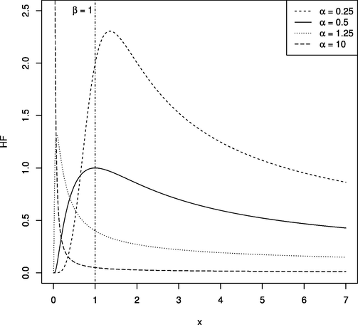
The HF for the LBS distribution with different values for $\alpha$ and $\beta =1$ .

Export to PPT

4 Critical value estimation

In the previous section, we established that the HF of the LBS distribution has either a unimodal or a decreasing curve. Thus, it is then of natural interest to determine the corresponding critical point $c_{\alpha ,\beta }$ . Based on Theorem 1, $c_{\alpha ,\beta }$ can be obtained as the solution of $g(x\text{;}\alpha ,\beta )$ which was given by (6). Nevertheless, the solution depends on the model parameters, which need to be estimated first. We propose to estimate them using the modified moments estimation method proposed by Ng et al. (2003), who noticed that the MMEs are easier to use than the maximum likelihood estimators (MLEs) and both share similar behaviors. Let $x_1,\dots ,x_n$ represent an observed random sample of size n from the LBS distribution with PDF as in (4). For the critical value $c_{\alpha ,\beta }$ , the MME is simply $c_{\tilde{\alpha },\tilde{\beta }}=\tilde{c}$ , such that $\tilde{\alpha }=\sqrt{\left(\frac{6}{{\pi }^2}\left[\sqrt{\left(\frac{s}{r}\right)}-1\right]\right)}$ and $\tilde{\beta }=\sqrt{\mathit{sr}}$ are the MMEs of $\alpha$ and $\beta$ , respectively, where $s=n^{-1}{\sum }_i^n{x}_i$ and $r^{-1}=n^{-1}{\sum }_i^n{x}_i^{-1}$ .

Clearly, the MME of $c_{\alpha ,\beta }$ does not have an explicit expression; therefore, we seek to obtain a functional approximation of $c_{\alpha ,\beta }$ as a function of the model parameters $\alpha$ and $\beta$ . By following the same approach as in Kundu et al. (2008), we obtain an approximated MME (AMME) for $c_{\alpha ,\beta }$ as follows. Recall that $\beta$ is a scale parameter; thus, it is obvious that since $c_{\alpha ,\beta }$ is the critical point of the HF of the LBS distribution, then $c_{\alpha ,\beta }$ = $\beta c_{\alpha ,1}$ . By using Box-Cox transformation, we observed that ${\left[c_{\alpha ,1}\right]}^{-0.5}$ is approximately a linear function of $\alpha$ and so a reasonably good approximation of $\beta c_{\alpha ,1}$ ; say, $c_{\alpha ,1}^{\ast }$ is given by $c_{\alpha ,1}^{\ast }={(-0.47633+3.22458\alpha )}^{-2}$ given that the actual value of $\alpha$ is approximately greater than 0.15. Accordingly, the AMME of $c_{\alpha ,\beta }^{\ast }$ is simply $c_{\tilde{\alpha },\tilde{\beta }}^{\ast }={\tilde{c}}^{\ast }=\tilde{\beta }{(-0.47633+3.22458\alpha )}^{-2}$ .

5 Simulation outcomes

This section reports the outcomes of a Monte Carlo simulation study which have been conducted to numerically examine the estimation efficiency of the proposed estimators mentioned in the preceding section assuming different values for the shape parameter and various sample sizes. The simulation outcomes are reported up to three decimal digits in Table 1 since they are computed based on $M=10,000$ simulation runs. The latter simulation runs provides an accuracy of the order $\pm {(10,000)}^{-0.5}=\pm 0.01$ (Karian and Dudewicz, 1999). The considered sample sizes were $n=25,50,75,100,250,500$ and $\alpha =0.5,1.0$ and $2.0$ as the values of the shape parameter. Without loss of any generality, we set the scale parameter $\beta =1$ for all cases. According to the chosen values of the model parameters, the values of the critical point $c_{\alpha ,\beta }$ are obtained by solving expression (6) after equating it to 0. It is to be noted that all computations were performed using an R program which is available upon request from the authors.

The MME and AMME are then obtained for $c_{\alpha ,\beta }$ , and for each estimate, we obtained the bias, the root-mean-squared error (RMSE), the average absolute difference between the true and estimate hazard functions ( $D_{\mathrm{abs}}$ ) and the maximum absolute difference between the true and estimate hazard functions ( $D_{\max }$ ), respectively, as $$\mathrm{Bias}(\tilde{c})=\frac{1}{M}{\displaystyle \sum _{i=1}^M}({\tilde{c}}_i-c_{\alpha ,\beta }),\mathrm{Bias}({\tilde{c}}^{\ast })=\frac{1}{M}{\displaystyle \sum _{i=1}^M}({\tilde{c}}_i^{\ast }-c_{\alpha ,\beta }),$$ $$\mathrm{RMSE}(\tilde{c})=\sqrt{\frac{1}{M}{\displaystyle \sum _{i=1}^M}{({\tilde{c}}_i-c_{\alpha ,\beta })}^2},\mathrm{RMSE}({\tilde{c}}^{\ast })=\sqrt{\frac{1}{M}{\displaystyle \sum _{i=1}^M}{({\tilde{c}}_i^{\ast }-c_{\alpha ,\beta })}^2},$$ $$D^{\mathrm{abs}}(\tilde{c})=D_1^{\mathrm{abs}}=\frac{1}{M}{\displaystyle \sum _{i=1}^M}\left|h(c_{\alpha ,\beta }\text{;}\alpha ,\beta )-h({\tilde{c}}_i\text{;}{\tilde{\alpha }}_i,{\tilde{\beta }}_i)\right|$$ $$D^{\mathrm{abs}}({\tilde{c}}^{\ast })=D_2^{\mathrm{abs}}=\frac{1}{M}{\displaystyle \sum _{i=1}^M}\left|h(c_{\alpha ,\beta }\text{;}\alpha ,\beta )-h({\tilde{c}}_i^{\ast }\text{;}{\tilde{\alpha }}_i,{\tilde{\beta }}_i)\right|$$ $$D^{\max }(\tilde{c})=D_1^{\max }={\displaystyle \underset{i=1,\dots ,M}{\max }}\left|h(c_{\alpha ,\beta }\text{;}\alpha ,\beta )-h({\tilde{c}}_i\text{;}{\tilde{\alpha }}_i,{\tilde{\beta }}_i)\right|$$ and $$D^{\max }({\tilde{c}}^{\ast })=D_2^{\max }={\displaystyle \underset{i=1,\dots ,M}{\max }}\left|h(c_{\alpha ,\beta }\text{;}\alpha ,\beta )-h({\tilde{c}}_i^{\ast }\text{;}{\tilde{\alpha }}_i,{\tilde{\beta }}_i)\right|$$ such that ${\tilde{\alpha }}_i,{\tilde{\beta }}_i$ are the MME of $\alpha$ and $\beta$ based on simulation run i, while ${\tilde{c}}_i$ ( ${\tilde{c}}_i^{\ast }$ ) is the MME (AMME) of $c_{\alpha ,\beta }$ . Table 1 summarizes the simulation study outcomes and reveals that MME and AMME of $c_{\alpha ,\beta }$ become more efficient as the sample size increases. Overall, when the shape parameter is small, namely, when $\alpha ⩽0.5$ , then the AMME is not performing very well; however, it is more accurate when $\alpha$ is large. As the values of both the sample size and the shape parameter increase, the MME and AMME of $c_{\alpha ,\beta }$ are quite similar in terms of the considered comparison criteria.

6 Application

This section reports the analysis of a real data set considered by Kundu et al. (2008) to compare between the BS distribution and the LBS distribution. The data consists of the lifetimes of Cavia Porcellus (guinea pigs) induced with different dosages of Mycobacterium Tuberculosis. For this data set, 72 observations are listed in Table 2.

We first estimate the model parameters of both the BS and the LBS distributions and both the MMEs and AMMEs of the critical values of the corresponding hazard functions, then we calculate several explanatory data analysis (EDA) measurements based on the considered data set as well as their approximations based on the estimated model parameters. Moreover, we test the fitted models’ suitability to the data using Anderson–Darling (AD) and Cramér-von Mises (CvM) goodness-of-fit tests. Finally, we evaluate the fitted hazard rates using the TTT method.

Table 3 summarizes the estimators of the model parameters and the critical values as well as the corresponding goodness-of-fit statistics, while Table 4 shows the outcomes of EDA measurements. By examining these tables, one can observe that the LBS distribution provided EDA measurements close to those of the observed sample compared to the BS distribution. Furthermore, both AD and CVM goodness-of-fit tests indicated that the LBS distribution is much more suitable for the considered data. Fig. 2 shows the histogram of the data compared to the fitted PDFs.

Close

Fig. 2

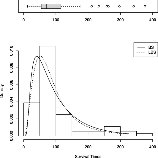
Histogram of the lifetimes of Cavia Porcellus vs. the fitted models.

Export to PPT

As indicated above, we used the TTT curve method to compare the LBS distribution and the BS distribution in terms of hazard rates. The empirical TTT curve is given by $W_X(u)=H_X^{-1}(u)/H_X^{-1}(1)$ , for $u\in (0,1)$ , such that $H_X^{-1}(u)={\int }_0^{F_X^{-1}(u)}[1-F_X(y)]\mathit{dy}$ , where $F_X^{-1}(·)$ is the quantile function of a lifetime random variable X. Fig. 3 shows the empirical scaled TTT plot based on the analyzed data alongside the fitted TTT curves of BS and LBS distributions. Since the fitted TTT curves are quite similar, we calculated the average and the maximum absolute differences between the empirical TTT curve and their fitted counterparts of the considered models. For the LBS distribution, the mean and maximum differences were 0.033 and 0.07, respectively, compared to 0.039 and 0.09 for the mean and maximum differences in the case of the BS distribution. The previous results support that the claim that the LBS distribution seems to provide a better fit to the Cavia Porcellus data than the BS distribution.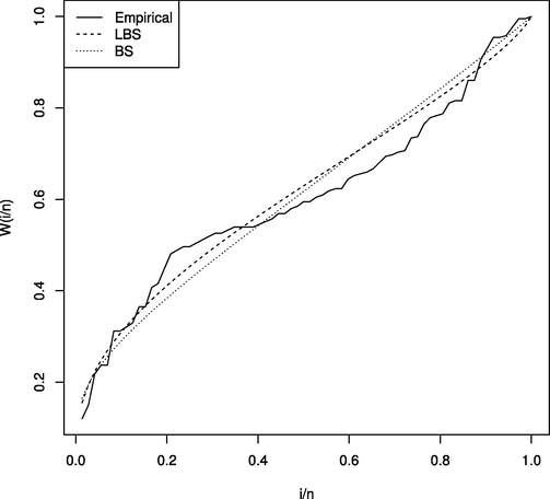

Close

Fig. 3

The fitted TTT curves and the empirical TTT curve based on the lifetimes of Cavia Porcellus..

Export to PPT

7 Conclusions

Studying the hazard rate is common in many scientific fields that involve reliability or survival analyses. In statistical literature, researchers might use the BS distribution instead of the lognormal and the inverse Gaussian distributions to model unimodal hazard rates. This study has revealed that the LBS distribution might be more flexible than the BS distribution since the corresponding HF curve can be either decreasing or unimodal. The behavior of the HF mainly depends on the value of the shape parameter alpha. The critical point of the hazard function, which represents the highest point of the peak of the hazard rate, has been estimated using two estimators based on the moment estimation methodology. Determining the critical point of the HF is vital to researchers since it may reduce any potential costs due to unnecessary interventions to the phenomenon of interest. Based on the Monte Carlo simulation study outcomes, the obtained estimators of the critical points, namely, MME and AMME, performed well as the sample size increases. Both become similar in estimation efficiency for large values of the shape parameter. Therefore, since the AMME of the critical value of the HF has a simple explicit form, we recommend using it given that the actual value of the shape parameter is greater than 0.15. Finally, based on a real data analysis, it is concluded that the LBS distribution might provide a better fit to real-life data compared to the well-known BS distribution. Therefore, The LBS distribution should be considered one of the lifetime distributions used to model either decreasing or unimodal hazard rates.

Several research directions need further investigation in the future. First, one can obtain different point estimators for the critical point of the HF in the case of the LBS distribution. The statistical literature is rich with other frequentist estimation methods (e.g., least-squares methods) and the Bayesian estimation approach. Thus, one may consider conducting a comparative study to examine these methods’ performances numerically. Assuming some censoring in the data is another potential research problem that needs to be addressed. A final research area that one might consider is obtaining the asymptotic joint distributions of different estimators and accordingly derive asymptotic confidence intervals compared to bootstrap confidence intervals in terms of lengths and coverage probabilities.

References

- How to identify a bathtub hazard rate. IEEE Transactions on Reliability. 1987;R-36:106-108.
- [Google Scholar]
- Shape and change point analyses of the Birnbaum–Saunders–t hazard rate and associated estimation. Computational Statistics and Data Analysis. 2012;56:3887-3897.
- Birnbaum-saunders distribution: A review of models, analysis, and applications. Applied Stochastic Models in Business and Industry. 2019;35:4-49.
- Acceptance sampling plans from truncated life tests based on the generalized birnbaum–saunders distribution. Communications in Statistics – Simulation and Computation. 2007;36:643-656.
- A proof of the shape of the Birnbaum-Saunders hazard rate function. Mathematical Sciences. 2008;33:49-56.
- The Birnbaum-Saunders autoregressive conditional duration model. Mathematics and Computers in Simulation. 2010;80:2062-2078.
- A new family of life distributions. Journal of Applied Probability. 1969;6:319-327.
- Control charts for monitoring the median parameter of birnbaum-saunders distribution. Quality and Reliability Engineering International. 2020;36:1333-1363.
- Stochastic models of failure in random environments. Canadian Journal of Statistics. 1985;13:171-183.
- A new family of life distributions based on the elliptically contoured distributions. Journal of Statistical Planning and Inference. 2005;128:445-457.
- Diáz-Garciá, J.A., Leiva-Sánchez, V., 2007. Erratum to A new family of life distributions based on the elliptically contoured distributions: [J. Statist. Plann. Inference, 128 (2), (2005) 445–457]. Journal of Statistical Planning and Inference 137, 1512–1513.
- A new five-parameter birnbaum–saunders distribution for modeling bicoid gene expression data. Mathematical Biosciences. 2020;319:108275
- Continuous Univariate Distributions. Vol vol. 2. John Wiley & Sons. 2nd Ed.; 1995.
- Economic design of repetitive group sampling plan based on truncated life test under birnbaum–saunders distribution. Communications in Statistics – Simulation and Computation 2020:1-17.
- Modern Statistical Systems and GPSS Simulations. CRC Press (2nd Ed.). 1999.
- On the hazard function of Birnbaum-Saunders distribution and associated inference. Computational Statistics & Data Analysis. 2008;52:2692-2702.
- Long–term survival of patients with breast cancer: a study of the curability of the disease. BMJ. 1979;2:1247-1251.
- Generalized birnbaum-saunders distributions applied to air pollutant concentration. Environmetrics. 2008;19:235-249.
- Accelerated Testing. John Wiley & Sons; 2009.
- Modified moment estimation for the two-parameter Birnbaum-Saunders distribution. Computational Statistics and Data Analysis. 2003;43:283-298.
- The generalized birnbaum–saunders distribution and its theory, methodology, and application. Communications in Statistics – Theory and Methods. 2008;37:645-670.
- On mean-based bivariate birnbaum-saunders distributions: Properties, inference and application. Communications in Statistics – Theory and Methods. 2019;49:6032-6056.