The extended Weibull distribution with its properties, estimation and modeling skewed data

Mashail M. Al Sobhi

doi:10.1016/j.jksus.2021.101801

View/Download PDF

Buy Reprints

PDF

Translate this page into:

Original article

02 2021

:34;

101801

doi:

10.1016/j.jksus.2021.101801

The extended Weibull distribution with its properties, estimation and modeling skewed data

Mashail M. Al Sobhi

Department of Mathematics, Umm-Al-Qura University, Makkah 24227, Saudi Arabia

Received: 2021-2-6, Accepted: 2021-12-22,

Disclaimer:
This article was originally published by Elsevier and was migrated to Scientific Scholar after the change of Publisher.

Abstract

The present article introduces a new distribution called the odd log–logistic Lindley-Weibull (OLLLW) distribution that provides greater flexibility in modeling data in applied areas such as medicine and engineering. The OLLLW model provides left-skewed, symmetric, right-skewed, and reversed-J shaped densities. Its hazard function can be bathtub, unimodal, increasing or decreasing. The OLLLW density was expressed as a linear mixture of Weibull densities. Some distributional properties of the introduced model are derived. Its parameters are estimated using five classical estimators called, the maximum likelihood, Anderson–Darling, least-squares, Cramér-von Mises, and weighted least squares estimators. The performance of the proposed estimators is explored by detailed simulation results. The flexibility of the OLLLW distribution is studied by two real data sets from medicine and engineering sciences, showing that its capability to fit the data effectively than the Weibull, Fréchet Weibull, transmuted Weibull, gamma Weibull, transmuted exponentiated Weibull, and modified Weibull distributions.

Keywords

Anderson–Darling estimators

Cramér-von Mises estimation

Moments

odd log–logistic Lindley family

Simulation

Weibull distribution

60E05

62F10

1 Introduction

Recently, many researchers proposed different ways for generating new extended distributions to enhance and increase its capability to model diverse lifetime data which have a high degree of skewness and kurtosis. These extended distributions can provide more flexibility in modeling several data sets in practice. The exponential, generalized exponential, Weibull, and gamma distributions are adopted for modeling monotonic hazard rates over other models. However, these models are not reasonable for modeling non-monotone hazard rates such as the unimodal and bathtub-shaped hazard rates. The distributions that provide bathtub or/and upside-down bathtub failure rates are very useful in survival and reliability analysis (Kotz et al., 2000).

Several models were proposed to model real lifetime data such as the Weibull distribution as one of the most important distributions for this purpose. Further, the Weibull distribution is adopted to generate families of distributions such as the Weibull-G family Bourguignon et al. (2014), exponentiated Weibull-H family Cordeiro et al. (2017), extended odd Weibull-G family Alizadeh et al. (2018), Weibull Marshall-Olkin family Korkmaz et al. (2019), and new extended-X family by Zichuan et al. (2020), and new Weibull-X family by Ahmad et al. (2018), among others.

Recently many authors proposed several extended versions and generalizations of the Weibull distribution to increase its flexibility. For example, exponentiated-Weibull by Mudholkar and Srivastava (1993), extended-Weibull by Marshall and Olkin (1997), modified Weibull by Xie et al. (2002), beta-Weibull by Lee et al. (2007), Kumaraswamy-Weibull by Cordeiro et al. (2010), truncated-Weibull by Zhang and Xie (2011), new extended-Weibull by Peng et al. (2014), alpha logarithmic transformed-Weibull by Nassar et al. (2018) Nassar et al. (2018), Kumaraswamy complementary Weibull geometric by Afify et al. (2017), Weibull-Weibull by Abouelmagd et al. (2017), odd log–logistic exponentiated-Weibull by Afify et al. (2018), alpha power exponentiated-Weibull by Mead et al. (2019), odd Lomax-Weibull by Cordeiro et al. (2019), new extended Weibull by Elbatal et al. (2019), Marshall-Olkin power generalized Weibull by Afify et al. (2020), odd Dagum-Weibull by Afify et al. (2020), extended inverse Weibull by Alkarni et al. (2020), logarithmic transformed Weibull by Nassar et al. (2020), and arcsine exponentiated-Weibull distributions by He et al. (2020).

In this article, we propose a new extension of the Weibull distribution, referred to as the log–logistic Lindley-Weibull (OLLLW) distribution which contains the log–logistic Lindley-exponential and log–logistic Lindley-Rayleigh distributions as special cases. The OLLLW distribution can be considered as a suitable model for modeling skewed data encountered in different applied fields such as biomedical studies, public health, engineering, and survival and reliability analysis. The OLLLW density can be viewed as a mixture of Weibull densities. The OLLLW distribution exhibits monotone, increasing and decreasing, as well as non-monotone, unimodal and bathtub, hazard rates which makes it a superior to other lifetime distributions, which exhibit only increasing or/and decreasing, constant hazard rates. The OLLLW distribution outperforms many common lifetime distributions with respect to real data examples from medicine and engineering sciences.

Furthermore, we study how different classical estimators of the OLLLW parameters perform for several sample sizes and several parameter combinations. The studied classical estimation methods include the maximum likelihood estimators (MLE), least-squares estimators (LSE), Anderson Darling estimators (ADE), weighted least squares estimators (WLSE), and Cramér–von Mises estimators (CVME). The statistical literature contains comprehensive comparisons of different estimation methods for many distributions, such as the quasi xgamma-geometric Sen et al. (2019), Weibull Marshall-Olkin Lindley Afify et al. (2020), odd exponentiated half-logistic exponential Aldahlan and Afify (2020), alpha power exponentiated exponential Afify et al. (2020), generalized Ramos-Louzada Al-Mofleh et al. (2020), and logarithmic transformed Weibull Nassar et al. (2020) distributions.

The OLLLW model is constructed using the odd log–logistic Lindley-G (OLLLi-G) family (Alizadeh et al. Alizadeh et al. (2020)) which is defined by the following cumulative distribution function (CDF)

(1)

F (x) = \frac{{\{1 - (1 + \frac{θ}{θ + 1} \frac{G (x; φ)}{\overline{G} (x; φ)}) e^{- \frac{θ G (x; φ)}{\overline{G} (x; φ)}}\}}^{α}}{{\{1 - (1 + \frac{θ}{θ + 1} \frac{G (x; φ)}{\overline{G} (x; φ)}) e^{- \frac{θ G (x; φ)}{\overline{G} (x; φ)}}\}}^{α} + {\{(1 + \frac{θ}{θ + 1} \frac{G (x; φ)}{\overline{G} (x; φ)}) e^{- \frac{θ G (x; φ)}{\overline{G} (x; φ)}}\}}^{α}},

where

G (x; φ)

denotes a baseline CDF with parameters vector

φ, α > 0

and

θ > 0

The corresponding probability density function (PDF) of (1) is

(2)

f (x; α, θ, φ) = \frac{\frac{α θ^{2} g (x; φ)}{(1 + θ) \overline{G} {(x; φ)}^{3}} e^{- \frac{θ G (x; φ)}{\overline{G} (x; φ)}} {(1 + \frac{θ}{θ + 1} \frac{G (x; φ)}{\overline{G} (x; φ)})}^{α - 1} {\{1 - (1 + \frac{θ}{θ + 1} \frac{G (x; φ)}{\overline{G} (x; φ)}) e^{- \frac{θ G (x; φ)}{\bar{G} (x; φ)}}\}}^{α - 1}}{{({\{1 - (1 + \frac{θ}{θ + 1} \frac{G (x; φ)}{\overline{G} (x; φ)}) e^{- \frac{θ G (x; φ)}{\overline{G} (x; φ)}}\}}^{α} + {\{(1 + \frac{θ}{θ + 1} \frac{G (x; φ)}{\bar{G} (x; φ)}) e^{- \frac{θ G (x; φ)}{\overline{G} (x; φ)}}\}}^{α})}^{2}},

where

g (x; φ)

is a baseline density with a vector of parameters

φ

The paper is organized as follows. In Section 2, we introduce the OLLLW distribution. The properties of the OLLLW distribution are discussed Section 3. Section 4 presents five methods of estimation. In Section 5, detailed simulation results are presented to compare the performance of these estimation methods. In Section 6, the importance of the OLLLW distribution is discussed by two real data sets. Finally, some concluding remarks are given in Section 7.

2 The OLLLW distribution

The CDF of the OLLLW distribution follows, by inserting the CDF and survival function (SF) of the Weibull distribution in Eq. (1), for $x > 0$ and $λ, β, α, θ > 0$ ) as

(3)

F (x) = {({\{\frac{e^{θ - θ e^{{(λ x)}^{β}}} [θ e^{{(λ x)}^{β}} + 1]}{θ + 1}\}}^{α} {\{1 - \frac{e^{θ - θ e^{{(λ x)}^{β}}} [θ e^{{(λ x)}^{β}} + 1]}{θ + 1}\}}^{- α} + 1)}^{- 1} .

The PDF of the OLLLW model takes the form

(4)

f (x) = \frac{α β θ^{2} {(θ + 1)}^{1 - 2 α} λ^{β} x^{β - 1} {([θ e^{{(λ x)}^{β}} + 1] \{(θ + 1) e^{θ e^{{(λ x)}^{β}}} - e^{θ} [θ e^{{(λ x)}^{β}} + 1]\})}^{α - 1}}{{({\{\frac{e^{θ - θ e^{{(λ x)}^{β}}} [θ e^{{(λ x)}^{β}} + 1]}{θ + 1}\}}^{α} + {\{1 - \frac{e^{θ - θ e^{{(λ x)}^{β}}} [θ e^{{(λ x)}^{β}} + 1]}{θ + 1}\}}^{α})}^{2} e^{- [α θ + (θ - 2 α θ) e^{{(λ x)}^{β}} + 2 {(λ x)}^{β}]}} .

The SF and hazard rate function (HRF) of the OLLLW distribution have the forms

(5)

S (x) = \frac{1}{e^{- α θ} {(\frac{(θ + 1) e^{θ e^{{(λ x)}^{β}}}}{θ e^{{(λ x)}^{β}} + 1} - e^{θ})}^{α} + 1},

(6)

h (x) = α β θ^{2} {(θ + 1)}^{1 - 2 α} λ^{β} x^{β - 1} {([θ e^{{(λ x)}^{β}} + 1] \{(θ + 1) e^{θ e^{{(λ x)}^{β}}} - e^{θ} [θ e^{{(λ x)}^{β}} + 1]\})}^{α - 1}

(7)

\times \frac{\{e^{- α θ} {[\frac{(θ + 1) e^{θ e^{{(λ x)}^{β}}}}{θ e^{{(λ x)}^{β}} + 1} - e^{θ}]}^{α} + 1\} e^{[α θ + (θ - 2 α θ) e^{{(λ x)}^{β}} + 2 {(λ x)}^{β}]}}{{({\{\frac{e^{θ - θ e^{{(λ x)}^{β}}} [θ e^{{(λ x)}^{β}} + 1]}{θ + 1}\}}^{α} + {\{1 - \frac{e^{θ - θ e^{{(λ x)}^{β}}} [θ e^{{(λ x)}^{β}} + 1]}{θ + 1}\}}^{α})}^{2}} .

Plots of the PDF and HRF of the OLLLW distribution are shown in Figs. 1 and 2, respectively. These plots show that the OLLLW distribution can provide left-skewed, symmetrical, right-skewed or reversed-J shaped densities, and its HRF exhibits bathtub, decreasing, unimodel, increasing, J shaped or reversed-J shaped hazard rates.

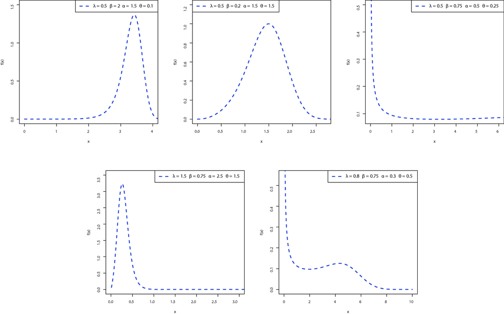
Some possible shapes of the PDF of the OLLLW distribution.

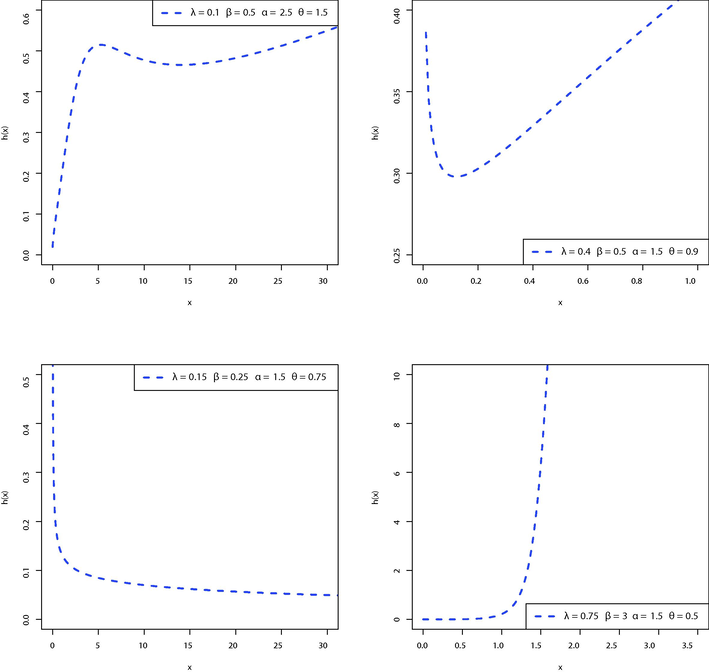
Some possible shapes of the HRF of the OLLLW distribution.

3 Mathematical Properties

3.1

3.1 Linear Representation

By using Eq. (10) introduced by Alizadeh et al. Alizadeh et al. (2020), we have $f (x) = \sum_{k, s, m = 0}^{\infty} \sum_{l = 0}^{r} \sum_{r = 0}^{k} w_{k, r, s, l, m} (s + l + m + 1) g (x) G {(x)}^{s + l + m},$ then by using the binomial expansion ${(1 - z)}^{b} = \sum_{j = 0}^{\infty} {(- 1)}^{j} (\begin{matrix} b \\ j \end{matrix}) z^{j}$ , we have $\begin{matrix} f (x) = & \sum_{k, s, m = 0}^{\infty} \sum_{l = 0}^{r} \sum_{r = 0}^{k} w_{k, r, s, l, m} (s + l + m + 1) β λ^{β} x^{β - 1} e^{- {(λ x)}^{β}} {[1 - e^{- {(λ x)}^{β}}]}^{s + l + m} \\ = & \sum_{k, s, m = 0}^{\infty} \sum_{l = 0}^{r} \sum_{r = 0}^{k} \sum_{j = 0}^{\infty} {(- 1)}^{j} (\begin{matrix} s + l + m \\ j \end{matrix}) w_{k, r, s, l, m} (s + l + m + 1) β λ^{β} x^{β - 1} e^{- λ^{β} (j + 1) x^{β}} \\ = & \sum_{j = 0}^{\infty} Φ_{j} q_{j} (x), \end{matrix}$ where $Φ_{j} = Φ (k, s, m, l, r) = \sum_{k, s, m = 0}^{\infty} \sum_{l = 0}^{r} \sum_{r = 0}^{k} {(- 1)}^{j} \frac{(s + l + m + 1)}{j + 1} (\begin{matrix} s + l + m \\ j \end{matrix}) w_{k, r, s, l, m}$ and $q_{j} (x)$ is the PDF of Weibull distribution with shape parameter $β$ and scale parameter $λ {(j + 1)}^{\frac{1}{β}}$ .

3.2

3.2 Moments

The rth moments of the OLLLW distribution has the form $μ_{r}^{'} = E (X^{r}) = \int_{0}^{\infty} x^{r} f (x) dx = \sum_{j = 0}^{\infty} Φ_{k, s, m, l, r, j} {[λ {(j + 1)}^{\frac{1}{β}}]}^{- r} Γ (1 + \frac{r}{β}) .$ Setting $r = 1, 2, 3$ , and 4, respectively, we obtain the first four moments about the origin of the OLLLW distribution.

The nth central moment of X, say $μ_{n}$ , follows as $μ_{n} = E {(x - μ)}^{n} = \sum_{k = 0}^{\infty} {(- 1)}^{k} (\begin{matrix} n \\ k \end{matrix}) μ_{1}^{' k} μ_{n - k}^{'} .$ The cumulants ( $k_{n}$ ) of X can be obtained as the following $k_{n} = μ_{n}^{'} - \sum_{r = 0}^{n - 1} (\begin{matrix} n - 1 \\ r - 1 \end{matrix}) k_{r} μ_{n - r}^{'} .$

3.3

3.3 Incomplete Moments

The sth incomplete moment of Weibull distribution is $I_{s} = γ^{- s} B (1 + \frac{s}{β}, {(γ t)}^{β}),$ where $B (s, t)$ is lower incomplete gamma function.

The sth incomplete moments of the OLLLW distribution is $Ψ_{s} (t) = \int_{0}^{t} x^{s} f (x) dx = \sum_{j = 0}^{\infty} Φ_{k, s, m, l, r, j} {[λ^{β} (j + 1)]}^{- s} B (1 + \frac{s}{β}, {(λ {(j + 1)}^{\frac{1}{β}} t)}^{β}) .$ The mean residual life of the OLLLW distribution is $m_{x} (t) = \frac{1 - Ψ_{1} (t)}{R (t) - t} .$ The mean inactivity time of the OLLLW distribution is $M_{x} (t) = t - \frac{Ψ_{1} (t)}{F (t)} .$

3.4

3.4 Generating Function

the moment generating function (MGF) of Weibull distribution is given by $M (t) = \int_{0}^{\infty} e^{tx} f (x) dx = β γ^{β} \int_{0}^{\infty} e^{tx} x^{β - 1} e^{- {(γ x)}^{β}} dx,$ By expanding the first exponential and calculating the integral, we can write $M (t) = \sum_{m = 0}^{\infty} \frac{{(t / γ)}^{m}}{m!} Γ (β + m / β) .$ Consider the Wright generalized hyper geometric function which is defined by $_{p} Ω_{q} [\begin{matrix} (γ_{1}, A_{1}), \dots, (γ_{p}, A_{p}) \\ (β_{1}, B_{1}), \dots, (β_{q}, B_{q}) \end{matrix}; x] = \sum_{n = 0}^{\infty} \frac{\prod_{j = 1}^{p} Γ (γ_{j} + A_{j} n) x^{n}}{\prod_{j = 1}^{q} Γ (β_{j} + B_{j} n) n!} .$ Hence, we can write the MGF as $M (t) =_{1} Ω_{0} [\begin{matrix} (1, - β^{- 1}) \\ - \end{matrix}; \frac{t}{γ}] .$ Hence, the MGF of the OLLLW model is given by $M (t) = \sum_{j = 0}^{\infty} {Φ_{k, s, m, l, r, j}}_{1} Ω_{0} [\begin{matrix} (1, - β^{- 1}) \\ - \end{matrix}; \frac{t}{λ {(j + 1)}^{\frac{1}{β}}}] .$ Characteristic function of the OLLLW distribution can be determined from the last equation by setting $t = it$ .

3.5

3.5 Order Statistics

The PDF and CDF of the $i th$ order statistic for the OLLLW distribution are $\begin{matrix} f_{i : n} (x) = & \frac{f (x)}{B (i, n - i + 1)} \sum_{h = 0}^{\infty} {(- 1)}^{h} (\begin{matrix} n - i \\ h \end{matrix}) F^{h + i - 1} (x) \\ = & \frac{\sum_{j = 0}^{\infty} Φ_{k, s, m, l, r, j} q_{j} (x)}{B (i, n - i + 1)} \sum_{h = 0}^{\infty} {(- 1)}^{h} (\begin{matrix} n - i \\ h \end{matrix}) \\ \times & {({\{\frac{e^{θ - θ e^{{(λ x)}^{β}}} [θ e^{{(λ x)}^{β}} + 1]}{θ + 1}\}}^{α} {\{1 - \frac{e^{θ - θ e^{{(λ x)}^{β}}} [θ e^{{(λ x)}^{β}} + 1]}{θ + 1}\}}^{- α} + 1)}^{- (h + i - 1)} . \end{matrix}$ where $B (., .)$ is beta function. $\begin{matrix} F_{i : n} (x) = & \sum_{r = i}^{n} (^{n}_{r}) {(F (x))}^{r} {(1 - F (x))}^{n - r} \\ = & \frac{Γ (n + 1)}{Γ (- i + n + 1)} {\{e^{α θ} {[\frac{(θ + 1) e^{θ e^{{(λ x)}^{β}}}}{θ e^{{(λ x)}^{β}} + 1} - e^{θ}]}^{- α} + 1\}}^{- i} {\{e^{- α θ} {[\frac{(θ + 1) e^{θ e^{{(λ x)}^{β}}}}{θ e^{{(λ x)}^{β}} + 1} - e^{θ}]}^{α} + 1\}}^{- n + i}_{2} {\tilde{Ω}}_{1} (1, i - n; i + 1; - {\{\frac{e^{[- 1 + e^{{(x λ)}^{β}}] θ} (θ + 1)}{e^{{(x λ)}^{β}} θ + 1} - 1\}}^{α}), \end{matrix}$ where $_{2} {\tilde{Ω}}_{1} (1, i - n; i + 1; - {\{\frac{e^{[- 1 + e^{{(x λ)}^{β}}] θ} (θ + 1)}{e^{{(x λ)}^{β}} θ + 1} - 1\}}^{α})$ is a hyper geometric regularized function.

4 Methods of Estimation

In this section, we discuss the estimation of the OLLLW parameters by different estimators including the MLE, ADE, CVME, LSE and WLSE.

4.1

4.1 Maximum Likelihood Estimation

Let $x_{1}, x_{2}, \dots, x_{n}$ be a random sample from the PDF (4), then the log-likelihood function reduces to

(8)

L = (β - 1) \sum_{i = 1}^{n} \log (x_{i}) + n \log (α β θ^{2} {(θ + 1)}^{1 - 2 α} λ^{β}) + \sum_{i = 1}^{n} (α θ + (θ - 2 α θ) e^{{(λ x_{i})}^{β}} + 2 {(λ x_{i})}^{β}) + (α - 1) \sum_{i = 1}^{n} \log (θ e^{{(λ x_{i})}^{β}} + 1) + (α - 1) \sum_{i = 1}^{n} \log ((θ + 1) e^{θ e^{{(λ x_{i})}^{β}}} - e^{θ} (θ e^{{(λ x_{i})}^{β}} + 1)) - 2 \sum_{i = 1}^{n} \log ({(\frac{e^{θ - θ e^{{(λ x_{i})}^{β}}} (θ e^{{(λ x_{i})}^{β}} + 1)}{θ + 1})}^{α} + {(1 - \frac{e^{θ - θ e^{{(λ x_{i})}^{β}}} (θ e^{{(λ x_{i})}^{β}} + 1)}{θ + 1})}^{α}) .

By differentiating Eq. (8) with respect to

α, β

and

λ

, respectively, equating to zero, and solving the previous equations, we obtain estimators of the OLLLW parameters by the MLE.

4.2

4.2 Ordinary Least-Squares and Weighted Least-Squares Estimators

Let $x_{1 : n}, x_{2 : n}, \dots, x_{2 : n}$ be the order statistics of a random sample of size n from the OLLLW distribution. Hence, we have the OLSE of the OLLLW parameters by minimizing the following equation: $O = \sum_{i = 1}^{n} {[F (x_{i : n}) - \frac{i}{n + 1}]}^{2},$ The OLSE of the OLLLW parameters can also be obtained by solving the following nonlinear equations: $\sum_{i = 1}^{n} \{F (x_{i : n}) - \frac{i}{n + 1}\} Δ_{s} (x_{i : n}) = 0, s = 1, 2, 3, 4,$ where $Δ_{1} (x_{i : n}) = \frac{\partial}{\partial α} F (x_{i : n}), Δ_{2} (x_{i : n}) = \frac{\partial}{\partial β} F (x_{i : n}), Δ_{3} (x_{i : n}) = \frac{\partial}{\partial θ} F (x_{i : n})$ , and $Δ_{4} (x_{i : n}) = \frac{\partial}{\partial λ} F (x_{i : n})$ .

The WLSE of the OLLLW parameters can be calculated by minimizing the following equation: $W = \sum_{i = 1}^{n} \frac{{(n + 1)}^{2} (n + 2)}{i (n - i + 1)} {[F (x_{i : n}) - \frac{i}{n + 1}]}^{2} .$ Furthermore, the WLSE of the OLLLW parameters follow by solving the following nonlinear equations: $\sum_{i = 1}^{n} \frac{{(n + 1)}^{2} (n + 2)}{i (n - i + 1)} [F (x_{i : n}) - \frac{i}{n + 1}] Δ_{s} (x_{i : n}) = 0 .$

4.3

4.3 Anderson–Darling Estimation

The ADE of the OLLLW parameters are obtained by minimizing the following equation: $A = - n - \frac{1}{n} \sum_{i = 1}^{n} (2 i - 1) [\log F (x_{i : n}) + \log S (x_{i : n})] .$ The ADE can also be calculated by solving the following nonlinear equations: $\sum_{i = 1}^{n} (2 i - 1) [\frac{Δ_{s} (x_{i : n})}{F (x_{i : n})} - \frac{Δ_{s} (x_{n + 1 - i : n})}{S (x_{n + 1 - i : n})}] = 0 .$

4.4

4.4 Cramér–von Mises Estimation

The CVME of OLLLW parameters are obtained by minimizing the following equation: $CV = \frac{1}{12 n} + \sum_{i = 1}^{n} {[F (x_{i : n}) - \frac{2 i - 1}{2 n}]}^{2},$ or by solving the following nonlinear equations $\sum_{i = 1}^{n} \{F (x_{i : n}) - \frac{2 i - 1}{2 n}\} Δ_{s} (x_{i : n}) = 0 .$

5 Simulation Results

This section is devoted to exploring the behavior of the previous estimation methods for estimating the OLLLW parameters based on a detailed simulation study. Some different sample sizes, $n = {20, 30, 50, 100, 200, 400}$ , are considered along with some different parametric values of $λ, β, α$ and $θ$ , where $λ = {0.5, 1.5, 3.5}, β = {0.25, 0.5, 0.75, 1.75}, α = {0.5, 1.5, 2.5}$ and $θ {0.5, 1.5, 2.5}$ . The simulations were repeated $N = 2000$ times, where the random samples are generated from the OLLLW distribution to determine the following measures such as, average estimates (AEs) with their associated mean square error (MSEs), average absolute biases (ABBs), and mean relative errors of the estimates (MREs) for all studied sample sizes and parameters combinations using the statistical R software©.

The ABBs, MSEs, and MREs are given by: $ABBs = \frac{1}{N} \sum_{i = 1}^{N} | \hat{ψ} - ψ |, MSEs = \frac{1}{N} \sum_{i = 1}^{N} {(\hat{ψ} - ψ)}^{2}, MREs = \frac{1}{N} \sum_{i = 1}^{N} | \hat{ψ} - ψ | / ψ,$ where $ψ = {(λ, β, α, θ)}^{'}$ .the simulation results include the AEs, MSEs, ABBs and MREs for the OLLLW parameters were obtained for the five estimation methods and reported in Tables 1–4 . It is noted that the estimates of the OLLLW parameters obtained using the five estimation methods are quite reliable and close to the true values of the parameters, showing small MSEs, ABBs and MREs in all parameter combinations. The five estimators, MLE, ADE, CVME, LSE and WLSE, show the consistency property, where the MSEs decrease as n increases for all considered parameter combinations. In summary, we can conclude that the MLE, ADE, CVME, LSE and WLSE approaches perform very good in estimating the parameters the OLLLW model.

Table 1 Simulation results of the AEs, ABBs, MSEs and MREs of the OLLLW distribution for (

λ = 0.5, β = 0.5, α = 0.5, θ = 0.5

n	Est.	Est. Par.	MLE	ADE	CVME	LSE	WLSE
20	AEs	$\hat{λ}$	0.37223	0.51074	0.55029	0.63779	0.97212
		$\hat{β}$	0.65793	0.54499	0.57692	0.53378	0.57701
		$\hat{α}$	0.52270	0.56383	0.54524	0.52665	0.53563
		$\hat{θ}$	0.71352	0.62252	0.62519	0.57207	0.83341
	ABBs	$\hat{λ}$	0.21138	0.23141	0.35266	0.33645	0.76128
		$\hat{β}$	0.18493	0.11925	0.17748	0.16140	0.21868
		$\hat{α}$	0.11798	0.13697	0.19243	0.18946	0.20673
		$\hat{θ}$	0.27923	0.24677	0.33873	0.31430	0.63312
	MSEs	$\hat{λ}$	0.06868	0.08729	0.13617	0.13933	0.91268
		$\hat{β}$	0.06639	0.03076	0.05331	0.04326	0.10101
		$\hat{α}$	0.03056	0.04216	0.06004	0.05726	0.10237
		$\hat{θ}$	0.12409	0.10255	0.14956	0.12441	0.67105
	MREs	$\hat{λ}$	0.42276	0.46282	0.64531	0.67290	1.52256
		$\hat{β}$	0.36986	0.23850	0.35496	0.32281	0.43736
		$\hat{α}$	0.23596	0.27395	0.38486	0.37893	0.41345
		$\hat{θ}$	0.55847	0.49354	0.65374	0.62175	1.30622
30	AEs	$\hat{λ}$	0.38296	0.49641	0.53979	0.60426	0.88481
		$\hat{β}$	0.61424	0.54051	0.56506	0.53475	0.57499
		$\hat{α}$	0.52219	0.54683	0.53903	0.52592	0.50547
		$\hat{θ}$	0.70172	0.62755	0.65368	0.60927	0.86915
	ABBs	$\hat{λ}$	0.18335	0.20960	0.31309	0.33148	0.70540
		$\hat{β}$	0.13172	0.09440	0.15693	0.14589	0.18752
		$\hat{α}$	0.08564	0.09803	0.16262	0.15973	0.14469
		$\hat{θ}$	0.24935	0.22346	0.32364	0.29692	0.60557
	MSEs	$\hat{λ}$	0.05706	0.07850	0.12006	0.13496	0.81529
		$\hat{β}$	0.04125	0.02244	0.04219	0.03564	0.06127
		$\hat{α}$	0.01898	0.02582	0.04422	0.04220	0.04033
		$\hat{θ}$	0.11310	0.09313	0.13341	0.11700	0.66178
	MREs	$\hat{λ}$	0.36669	0.41920	0.62618	0.66296	1.41080
		$\hat{β}$	0.26343	0.18879	0.31387	0.29178	0.37503
		$\hat{α}$	0.17128	0.19607	0.32524	0.31945	0.28937
		$\hat{θ}$	0.49869	0.44691	0.64727	0.59383	1.21114
50	AEs	$\hat{λ}$	0.39306	0.47858	0.53531	0.58913	0.77840
		$\hat{β}$	0.58001	0.53397	0.55464	0.53025	0.58495
		$\hat{α}$	0.51806	0.52813	0.52119	0.51285	0.49067
		$\hat{θ}$	0.67093	0.60877	0.65169	0.61320	0.88552
	ABBs	$\hat{λ}$	0.13175	0.14864	0.30883	0.32435	0.61053
		$\hat{β}$	0.09040	0.06684	0.12809	0.11680	0.17510
		$\hat{α}$	0.05425	0.06016	0.11940	0.11728	0.10472
		$\hat{θ}$	0.19068	0.16782	0.29954	0.28470	0.58576
	MSEs	$\hat{λ}$	0.03873	0.05339	0.11753	0.12927	0.65511
		$\hat{β}$	0.02578	0.01450	0.02843	0.02341	0.05181
		$\hat{α}$	0.00972	0.01217	0.02503	0.02380	0.01939
		$\hat{θ}$	0.08718	0.07044	0.12238	0.11163	0.64481
	MREs	$\hat{λ}$	0.26351	0.29727	0.61767	0.64871	1.22106
		$\hat{β}$	0.18079	0.13367	0.25617	0.23359	0.35020
		$\hat{α}$	0.10850	0.12032	0.23880	0.23455	0.20943
		$\hat{θ}$	0.38135	0.33564	0.59908	0.56940	1.17151
100	AEs	$\hat{λ}$	0.43693	0.47596	0.53570	0.57791	0.65754
		$\hat{β}$	0.53636	0.51950	0.55015	0.53402	0.56879
		$\hat{α}$	0.50769	0.50803	0.49923	0.49549	0.48535
		$\hat{θ}$	0.59155	0.55544	0.62674	0.59622	0.76327
	ABBs	$\hat{λ}$	0.06698	0.06741	0.29317	0.30538	0.45102
		$\hat{β}$	0.03795	0.02797	0.10406	0.09751	0.13486
		$\hat{α}$	0.01845	0.01885	0.07748	0.07719	0.07010
		$\hat{θ}$	0.09765	0.08068	0.26707	0.25408	0.42273
	MSEs	$\hat{λ}$	0.01846	0.02070	0.10874	0.11822	0.40129
		$\hat{β}$	0.00777	0.00488	0.01892	0.01666	0.03201
		$\hat{α}$	0.00206	0.00239	0.01055	0.01024	0.00777
		$\hat{θ}$	0.04373	0.03293	0.10275	0.09403	0.37701
	MREs	$\hat{λ}$	0.13395	0.13483	0.58634	0.61075	0.90205
		$\hat{β}$	0.07591	0.05593	0.20813	0.19502	0.26972
		$\hat{α}$	0.03689	0.03770	0.15496	0.15439	0.14019
		$\hat{θ}$	0.19529	0.16136	0.53414	0.50816	0.84545
200	AEs	$\hat{λ}$	0.48270	0.48961	0.53164	0.55683	0.57714
		$\hat{β}$	0.50990	0.50641	0.54171	0.53223	0.55620
		$\hat{α}$	0.50063	0.50052	0.49494	0.49322	0.48836
		$\hat{θ}$	0.52459	0.51536	0.60689	0.58806	0.69250
	ABBs	$\hat{λ}$	0.01730	0.01583	0.27122	0.27779	0.35175
		$\hat{β}$	0.00990	0.00704	0.09254	0.08849	0.10685
		$\hat{α}$	0.00308	0.00297	0.05785	0.05760	0.05027
		$\hat{θ}$	0.02478	0.01823	0.22915	0.22056	0.31578
	MSEs	$\hat{λ}$	0.00487	0.00429	0.09690	0.10238	0.26557
		$\hat{β}$	0.00188	0.00109	0.01325	0.01201	0.01897
		$\hat{α}$	0.00023	0.00025	0.00538	0.00530	0.00398
		$\hat{θ}$	0.01056	0.00703	0.07859	0.07338	0.21204
	MREs	$\hat{λ}$	0.03459	0.03166	0.54245	0.55558	0.70351
		$\hat{β}$	0.01980	0.01409	0.18507	0.17697	0.21371
		$\hat{α}$	0.00617	0.00593	0.11570	0.11520	0.10053
		$\hat{θ}$	0.04957	0.03646	0.45830	0.44111	0.63155
400	AEs	$\hat{λ}$	0.49937	0.49939	0.53569	0.55121	0.49936
		$\hat{β}$	0.50044	0.50036	0.52805	0.52258	0.54322
		$\hat{α}$	0.49993	0.49995	0.49392	0.49310	0.49304
		$\hat{θ}$	0.50100	0.50095	0.57092	0.55951	0.62871
	ABBs	$\hat{λ}$	0.00063	0.00061	0.23134	0.23418	0.23527
		$\hat{β}$	0.00044	0.00036	0.07262	0.07058	0.07707
		$\hat{α}$	0.00007	0.00005	0.04078	0.04081	0.03632
		$\hat{θ}$	0.00100	0.00095	0.18371	0.17947	0.21208
	MSEs	$\hat{λ}$	0.00020	0.00018	0.07736	0.07994	0.11972
		$\hat{β}$	0.00010	0.00007	0.00806	0.00759	0.01010
		$\hat{α}$	0.00000	0.00000	0.00271	0.00271	0.00209
		$\hat{θ}$	0.00050	0.00046	0.05470	0.05205	0.09328
	MREs	$\hat{λ}$	0.00125	0.00121	0.46268	0.46836	0.47055
		$\hat{β}$	0.00088	0.00072	0.14525	0.14117	0.15415
		$\hat{α}$	0.00014	0.00010	0.08156	0.08161	0.07264
		$\hat{θ}$	0.00200	0.00191	0.36742	0.35894	0.42417

Table 2 Simulation results of the AEs, ABBs, MSEs and MREs of the OLLLW distribution for (

λ = 0.5, β = 0.25, α = 2.5, θ = 1.5

n	Est.	Est. Par.	MLE	ADE	CVME	LSE	WLSE
20	AEs	$\hat{λ}$	0.60662	0.58062	0.60480	0.59165	0.60372
		$\hat{β}$	0.38281	0.33324	0.36076	0.33855	0.32811
		$\hat{α}$	2.12735	2.30821	2.25169	2.23353	2.26736
		$\hat{θ}$	1.94566	1.84618	1.88502	1.83063	1.81747
	ABBs	$\hat{λ}$	0.35295	0.37936	0.37244	0.38723	0.40001
		$\hat{β}$	0.14585	0.10963	0.13446	0.12526	0.11310
		$\hat{α}$	0.72387	0.66685	0.71679	0.74239	0.69585
		$\hat{θ}$	0.46381	0.41852	0.42103	0.39541	0.42251
	MSEs	$\hat{λ}$	0.14965	0.16473	0.16006	0.17014	0.17800
		$\hat{β}$	0.03855	0.02427	0.03388	0.02976	0.02490
		$\hat{α}$	0.68675	0.58697	0.66203	0.71097	0.63339
		$\hat{θ}$	0.22836	0.19951	0.20122	0.18486	0.19945
	MREs	$\hat{λ}$	0.70590	0.75871	0.74488	0.77446	0.80003
		$\hat{β}$	0.58338	0.43851	0.53783	0.50104	0.45240
		$\hat{α}$	0.28955	0.26674	0.28672	0.29696	0.27834
		$\hat{θ}$	0.30920	0.27901	0.28069	0.26361	0.28168
30	AEs	$\hat{λ}$	0.57553	0.56142	0.56486	0.56092	0.58151
		$\hat{β}$	0.35775	0.31403	0.34303	0.32729	0.31773
		$\hat{α}$	2.18043	2.36659	2.29935	2.28934	2.31682
		$\hat{θ}$	1.92034	1.81370	1.88002	1.83660	1.81784
	ABBs	$\hat{λ}$	0.33721	0.37049	0.36164	0.37358	0.39361
		$\hat{β}$	0.12234	0.09084	0.11753	0.11128	0.09965
		$\hat{α}$	0.68138	0.60885	0.68481	0.69667	0.65656
		$\hat{θ}$	0.45378	0.40992	0.41350	0.39233	0.42213
	MSEs	$\hat{λ}$	0.13980	0.15835	0.15327	0.16062	0.17102
		$\hat{β}$	0.02688	0.01679	0.02647	0.02376	0.01940
		$\hat{α}$	0.59416	0.48601	0.59620	0.62019	0.54451
		$\hat{θ}$	0.22160	0.19564	0.19844	0.18579	0.19915
	MREs	$\hat{λ}$	0.67442	0.74098	0.72328	0.74717	0.78722
		$\hat{β}$	0.48937	0.36335	0.47010	0.44513	0.39859
		$\hat{α}$	0.27255	0.24354	0.27393	0.27867	0.26262
		$\hat{θ}$	0.30252	0.27430	0.27567	0.26155	0.28142
50	AEs	$\hat{λ}$	0.53156	0.52859	0.54069	0.54574	0.54924
		$\hat{β}$	0.33227	0.30273	0.32414	0.31294	0.30297
		$\hat{α}$	2.25327	2.40549	2.33426	2.33746	2.39520
		$\hat{θ}$	1.88757	1.81115	1.85212	1.81235	1.80534
	ABBs	$\hat{λ}$	0.31748	0.35421	0.35998	0.36909	0.38035
		$\hat{β}$	0.09605	0.07845	0.09746	0.09285	0.08534
		$\hat{α}$	0.60962	0.57085	0.63606	0.63893	0.60944
		$\hat{θ}$	0.43523	0.40767	0.39665	0.38037	0.41695
	MSEs	$\hat{λ}$	0.12606	0.14828	0.15139	0.15980	0.16289
		$\hat{β}$	0.01798	0.01330	0.01927	0.01778	0.01473
		$\hat{α}$	0.48968	0.43010	0.51754	0.52650	0.47179
		$\hat{θ}$	0.21048	0.19181	0.18834	0.17739	0.19864
	MREs	$\hat{λ}$	0.63497	0.70841	0.71968	0.73925	0.76070
		$\hat{β}$	0.38418	0.31381	0.38983	0.37138	0.34135
		$\hat{α}$	0.24385	0.22834	0.25442	0.25557	0.24378
		$\hat{θ}$	0.29015	0.27178	0.26443	0.25358	0.27695
100	AEs	$\hat{λ}$	0.49688	0.54568	0.55172	0.56469	0.55990
		$\hat{β}$	0.30508	0.28811	0.31615	0.30864	0.29570
		$\hat{α}$	2.33352	2.41247	2.31595	2.32343	2.37830
		$\hat{θ}$	1.83147	1.74308	1.81700	1.78208	1.76966
	ABBs	$\hat{λ}$	0.28503	0.34351	0.35830	0.36792	0.37706
		$\hat{β}$	0.06935	0.05944	0.08804	0.08482	0.07109
		$\hat{α}$	0.49696	0.48371	0.60743	0.60602	0.54822
		$\hat{θ}$	0.40362	0.35723	0.38196	0.36595	0.39950
	MSEs	$\hat{λ}$	0.10827	0.14425	0.14930	0.15604	0.16140
		$\hat{β}$	0.00991	0.00786	0.01568	0.01461	0.01052
		$\hat{α}$	0.34879	0.32328	0.47267	0.47191	0.38506
		$\hat{θ}$	0.19202	0.16256	0.17874	0.16881	0.18310
	MREs	$\hat{λ}$	0.57006	0.68702	0.71659	0.73584	0.75412
		$\hat{β}$	0.27741	0.23775	0.35215	0.33928	0.28435
		$\hat{α}$	0.19878	0.19348	0.24297	0.24241	0.21929
		$\hat{θ}$	0.26908	0.23816	0.25464	0.24397	0.26633
200	AEs	$\hat{λ}$	0.46952	0.53347	0.54130	0.55761	0.55846
		$\hat{β}$	0.28388	0.27314	0.30165	0.29681	0.28224
		$\hat{α}$	2.40986	2.45782	2.34591	2.35310	2.41006
		$\hat{θ}$	1.77638	1.69180	1.78321	1.75370	1.72396
	ABBs	$\hat{λ}$	0.24461	0.29458	0.33986	0.34714	0.35044
		$\hat{β}$	0.04812	0.04446	0.07290	0.07104	0.05665
		$\hat{α}$	0.37204	0.38208	0.54866	0.54642	0.46543
		$\hat{θ}$	0.36257	0.32611	0.36465	0.35395	0.38061
	MSEs	$\hat{λ}$	0.08926	0.12005	0.13808	0.14292	0.14542
		$\hat{β}$	0.00493	0.00418	0.01053	0.00998	0.00610
		$\hat{α}$	0.21224	0.21573	0.38326	0.38029	0.27856
		$\hat{θ}$	0.17022	0.14664	0.16702	0.16069	0.17139
	MREs	$\hat{λ}$	0.48922	0.58916	0.67972	0.69428	0.70087
		$\hat{β}$	0.19249	0.17784	0.29159	0.28417	0.22659
		$\hat{α}$	0.14881	0.15283	0.21946	0.21857	0.18617
		$\hat{θ}$	0.24171	0.21740	0.24310	0.23597	0.25374
400	AEs	$\hat{λ}$	0.44691	0.53808	0.55211	0.56510	0.56397
		$\hat{β}$	0.27323	0.26307	0.28519	0.28221	0.27214
		$\hat{α}$	2.44607	2.48730	2.39294	2.39861	2.43828
		$\hat{θ}$	1.74363	1.63971	1.71920	1.69882	1.68089
	ABBs	$\hat{λ}$	0.20993	0.26812	0.32984	0.33697	0.33900
		$\hat{β}$	0.03557	0.03223	0.05731	0.05616	0.04545
		$\hat{α}$	0.26300	0.28064	0.45825	0.45652	0.37903
		$\hat{θ}$	0.32595	0.28731	0.34307	0.33580	0.36802
	MSEs	$\hat{λ}$	0.07275	0.10981	0.13339	0.13833	0.13961
		$\hat{β}$	0.00276	0.00233	0.00633	0.00602	0.00369
		$\hat{α}$	0.12468	0.13408	0.27307	0.27087	0.19427
		$\hat{θ}$	0.15112	0.12645	0.15352	0.14879	0.15984
	MREs	$\hat{λ}$	0.41986	0.53623	0.65968	0.67394	0.67801
		$\hat{β}$	0.14226	0.12892	0.22925	0.22464	0.18180
		$\hat{α}$	0.10520	0.11226	0.18330	0.18261	0.15161
		$\hat{θ}$	0.21730	0.19154	0.22872	0.22387	0.24535

Table 3 Simulation results of the AEs, ABBs, MSEs and MREs of the OLLLW distribution for (

λ = 3.5, β = 0.75, α = 1.5, θ = 2.5

n	Est.	Est. Par.	MLE	ADE	CVME	LSE	WLSE
20	AEs	$\hat{λ}$	3.57711	3.49269	3.51955	3.49103	3.50103
		$\hat{β}$	0.87859	0.80235	0.82525	0.78589	0.78077
		$\hat{α}$	1.46297	1.53845	1.55203	1.49161	1.52253
		$\hat{θ}$	3.03006	2.74771	2.81906	2.66580	2.65335
	ABBs	$\hat{λ}$	0.49528	0.47334	0.46764	0.46305	0.47471
		$\hat{β}$	0.19829	0.18195	0.19001	0.18907	0.18176
		$\hat{α}$	0.34083	0.35374	0.35820	0.36926	0.35542
		$\hat{θ}$	0.71318	0.59115	0.60660	0.54899	0.57486
	MSEs	$\hat{λ}$	0.25322	0.23250	0.22843	0.22574	0.23349
		$\hat{β}$	0.04570	0.03996	0.04255	0.04237	0.04020
		$\hat{α}$	0.14741	0.15747	0.16112	0.17123	0.16068
		$\hat{θ}$	0.82908	0.57485	0.63813	0.50113	0.52679
	MREs	$\hat{λ}$	0.14579	0.13524	0.13361	0.13230	0.13563
		$\hat{β}$	0.26439	0.24261	0.25335	0.25209	0.24235
		$\hat{α}$	0.22722	0.23583	0.23880	0.24617	0.23695
		$\hat{θ}$	0.28527	0.23646	0.24264	0.21960	0.22995
30	AEs	$\hat{λ}$	3.54434	3.48021	3.48944	3.47791	3.48086
		$\hat{β}$	0.86189	0.78799	0.80407	0.77495	0.77411
		$\hat{α}$	1.46098	1.55211	1.56165	1.51426	1.54771
		$\hat{θ}$	2.98947	2.70341	2.74405	2.63074	2.64750
	ABBs	$\hat{λ}$	0.47709	0.46473	0.46416	0.46200	0.47037
		$\hat{β}$	0.19286	0.17555	0.18317	0.18465	0.17937
		$\hat{α}$	0.31610	0.33989	0.34155	0.34946	0.34809
		$\hat{θ}$	0.68274	0.55341	0.53421	0.52160	0.55095
	MSEs	$\hat{λ}$	0.23450	0.22657	0.22679	0.22499	0.23008
		$\hat{β}$	0.04354	0.03776	0.04047	0.04050	0.03890
		$\hat{α}$	0.12995	0.14295	0.14620	0.15263	0.14961
		$\hat{θ}$	0.78596	0.49393	0.47391	0.42686	0.48991
	MREs	$\hat{λ}$	0.13631	0.13278	0.13262	0.13200	0.13182
		$\hat{β}$	0.25715	0.23407	0.24422	0.24620	0.23916
		$\hat{α}$	0.21074	0.22659	0.22770	0.23297	0.23206
		$\hat{θ}$	0.27310	0.22136	0.21368	0.20864	0.22038
50	AEs	$\hat{λ}$	3.48420	3.44891	3.46880	3.46706	3.42226
		$\hat{β}$	0.84124	0.77383	0.79097	0.76563	0.76170
		$\hat{α}$	1.46864	1.56256	1.55456	1.53940	1.57001
		$\hat{θ}$	2.93522	2.66253	2.70476	2.60559	2.62870
	ABBs	$\hat{λ}$	0.45557	0.46138	0.45818	0.45881	0.46743
		$\hat{β}$	0.18050	0.16962	0.17687	0.17914	0.17381
		$\hat{α}$	0.30481	0.33234	0.33565	0.33981	0.33697
		$\hat{θ}$	0.65419	0.52981	0.52216	0.51142	0.53310
	MSEs	$\hat{λ}$	0.22124	0.22465	0.22254	0.22223	0.22787
		$\hat{β}$	0.03932	0.03575	0.03798	0.03814	0.03644
		$\hat{α}$	0.12040	0.13672	0.13851	0.14234	0.13880
		$\hat{θ}$	0.68648	0.44853	0.44195	0.40228	0.44850
	MREs	$\hat{λ}$	0.13016	0.13182	0.13091	0.13109	0.13355
		$\hat{β}$	0.24067	0.22616	0.23583	0.23885	0.23175
		$\hat{α}$	0.20320	0.22156	0.22377	0.22654	0.22465
		$\hat{θ}$	0.26168	0.21193	0.20887	0.20457	0.21324
100	AEs	$\hat{λ}$	3.46434	3.49114	3.49617	3.48573	3.48138
		$\hat{β}$	0.82486	0.77743	0.79404	0.76735	0.77365
		$\hat{α}$	1.46594	1.53252	1.52438	1.53865	1.53659
		$\hat{θ}$	2.86677	2.63901	2.69151	2.59591	2.63248
	ABBs	$\hat{λ}$	0.43473	0.45539	0.45718	0.44898	0.46036
		$\hat{β}$	0.16379	0.15676	0.17323	0.17625	0.16600
		$\hat{α}$	0.28156	0.29216	0.31753	0.32566	0.30546
		$\hat{θ}$	0.61248	0.49417	0.52033	0.50297	0.52196
	MSEs	$\hat{λ}$	0.20712	0.22107	0.22125	0.21641	0.22330
		$\hat{β}$	0.03389	0.03136	0.03530	0.03653	0.03393
		$\hat{α}$	0.10289	0.11068	0.12231	0.12846	0.11785
		$\hat{θ}$	0.59312	0.38493	0.43046	0.37688	0.41540
	MREs	$\hat{λ}$	0.12421	0.13011	0.13059	0.12828	0.13153
		$\hat{β}$	0.21839	0.20902	0.22931	0.23499	0.22134
		$\hat{α}$	0.18770	0.19477	0.21169	0.21711	0.20364
		$\hat{θ}$	0.24499	0.19767	0.19155	0.20119	0.20878
200	AEs	$\hat{λ}$	3.45888	3.48395	3.49535	3.49008	3.48466
		$\hat{β}$	0.80864	0.77811	0.79329	0.76738	0.77812
		$\hat{α}$	1.46850	1.51662	1.50986	1.53413	1.51692
		$\hat{θ}$	2.81096	2.66719	2.70223	2.60960	2.66916
	ABBs	$\hat{λ}$	0.43699	0.44175	0.45634	0.44513	0.43977
		$\hat{β}$	0.13988	0.14369	0.17044	0.16312	0.15119
		$\hat{α}$	0.24322	0.26079	0.30074	0.29726	0.27266
		$\hat{θ}$	0.56029	0.51587	0.49363	0.49213	0.51789
	MSEs	$\hat{λ}$	0.20775	0.21188	0.22060	0.21323	0.21102
		$\hat{β}$	0.02645	0.02719	0.03494	0.03257	0.02912
		$\hat{α}$	0.07918	0.09152	0.11117	0.11094	0.09674
		$\hat{θ}$	0.49958	0.41744	0.42426	0.35570	0.40321
	MREs	$\hat{λ}$	0.12485	0.12621	0.13038	0.12718	0.12565
		$\hat{β}$	0.18651	0.19158	0.22725	0.21750	0.20159
		$\hat{α}$	0.16215	0.17386	0.20049	0.19817	0.18177
		$\hat{θ}$	0.22412	0.20635	0.17369	0.19485	0.20016
400	AEs	$\hat{λ}$	3.40977	3.49330	3.49301	3.49528	3.49212
		$\hat{β}$	0.79701	0.77285	0.78897	0.77691	0.77740
		$\hat{α}$	1.47092	1.50701	1.50078	1.50993	1.50195
		$\hat{θ}$	2.79809	2.64219	2.69488	2.65183	2.66125
	ABBs	$\hat{λ}$	0.40179	0.43012	0.43453	0.43481	0.41370
		$\hat{β}$	0.11238	0.11757	0.15228	0.14799	0.12648
		$\hat{α}$	0.18542	0.21003	0.25919	0.25921	0.22225
		$\hat{θ}$	0.51760	0.46092	0.44598	0.46982	0.48987
	MSEs	$\hat{λ}$	0.18786	0.20605	0.20719	0.20673	0.20246
		$\hat{β}$	0.01912	0.02001	0.02972	0.02824	0.02232
		$\hat{α}$	0.05192	0.06431	0.08804	0.08823	0.06930
		$\hat{θ}$	0.45702	0.34780	0.41094	0.31580	0.37366
	MREs	$\hat{λ}$	0.11480	0.12289	0.12415	0.12423	0.10677
		$\hat{β}$	0.14984	0.15676	0.20304	0.19732	0.16864
		$\hat{α}$	0.12361	0.14002	0.17279	0.17281	0.14817
		$\hat{θ}$	0.20704	0.18437	0.13065	0.16590	0.19595

Table 4 Simulation results of the AEs, ABBs, MSEs and MREs of the OLLLW distribution for (

λ = 1.5, β = 1.75, α = 1.5, θ = 2.5

n	Est.	Est. Par.	MLE	ADE	CVME	LSE	WLSE
20	AEs	$\hat{λ}$	1.67118	1.62893	1.62859	1.60130	1.63080
		$\hat{β}$	1.82043	1.67441	1.73593	1.65012	1.62134
		$\hat{α}$	1.52594	1.60519	1.60013	1.57086	1.59288
		$\hat{θ}$	2.25130	2.21103	2.24074	2.20566	2.15454
	ABBs	$\hat{λ}$	0.34568	0.38125	0.37960	0.40829	0.40482
		$\hat{β}$	0.26676	0.29186	0.27827	0.31683	0.32190
		$\hat{α}$	0.33449	0.36924	0.37299	0.39652	0.38300
		$\hat{θ}$	0.65242	0.72251	0.82364	0.67691	0.75381
	MSEs	$\hat{λ}$	0.14759	0.17231	0.17315	0.19398	0.18986
		$\hat{β}$	0.09753	0.11846	0.10261	0.14092	0.14742
		$\hat{α}$	0.14325	0.16749	0.17093	0.18795	0.17735
		$\hat{θ}$	0.52459	0.63664	0.55614	0.60349	0.69667
	MREs	$\hat{λ}$	0.25698	0.25417	0.25307	0.27219	0.26988
		$\hat{β}$	0.16823	0.16678	0.15901	0.18105	0.18394
		$\hat{α}$	0.22299	0.24616	0.24866	0.26435	0.25533
		$\hat{θ}$	0.26097	0.28900	0.46243	0.27076	0.40152
30	AEs	$\hat{λ}$	1.65463	1.60902	1.59409	1.58006	1.60762
		$\hat{β}$	1.78781	1.65221	1.70467	1.64036	1.62231
		$\hat{α}$	1.52835	1.61895	1.61149	1.59412	1.61250
		$\hat{θ}$	2.26799	2.24242	2.29199	2.25364	2.21051
	ABBs	$\hat{λ}$	0.33568	0.36597	0.36502	0.39227	0.38737
		$\hat{β}$	0.25254	0.28739	0.27746	0.30743	0.31532
		$\hat{α}$	0.30434	0.35184	0.35367	0.36822	0.36484
		$\hat{θ}$	0.64430	0.70017	0.79064	0.66879	0.72541
	MSEs	$\hat{λ}$	0.14009	0.16141	0.16207	0.18007	0.17463
		$\hat{β}$	0.92364	0.11598	0.10118	0.12767	0.13510
		$\hat{α}$	0.12293	0.15173	0.10036	0.16554	0.16126
		$\hat{θ}$	0.51302	0.62742	0.42523	0.57262	0.64078
	MREs	$\hat{λ}$	0.22378	0.24398	0.24335	0.26151	0.25825
		$\hat{β}$	0.14431	0.16799	0.15855	0.17568	0.18018
		$\hat{α}$	0.20290	0.23456	0.23578	0.24548	0.24322
		$\hat{θ}$	0.25772	0.28007	0.40243	0.26752	0.38103
50	AEs	$\hat{λ}$	1.62621	1.59909	1.58694	1.58518	1.59894
		$\hat{β}$	1.75500	1.62817	1.67240	1.62225	1.60466
		$\hat{α}$	1.53790	1.62917	1.61117	1.60751	1.63321
		$\hat{θ}$	2.30873	2.24960	2.29271	2.25148	2.23593
	ABBs	$\hat{λ}$	0.30329	0.35146	0.35242	0.37364	0.36282
		$\hat{β}$	0.25093	0.27385	0.27740	0.30245	0.31140
		$\hat{α}$	0.29121	0.33748	0.33737	0.34812	0.34765
		$\hat{θ}$	0.63464	0.69767	0.73956	0.57649	0.71817
	MSEs	$\hat{λ}$	0.12187	0.14992	0.15420	0.16805	0.15756
		$\hat{β}$	0.08031	0.11681	0.10319	0.12454	0.13453
		$\hat{α}$	0.11209	0.14306	0.14268	0.14960	0.14875
		$\hat{θ}$	0.50510	0.61742	0.40692	0.49496	0.63704
	MREs	$\hat{λ}$	0.20220	0.23431	0.23495	0.24910	0.24188
		$\hat{β}$	0.14339	0.16792	0.15851	0.17283	0.17795
		$\hat{α}$	0.19414	0.22499	0.22491	0.23208	0.23177
		$\hat{θ}$	0.25386	0.27907	0.31684	0.22085	0.32048
1000	AEs	$\hat{λ}$	1.62533	1.62120	1.60816	1.60981	1.62067
		$\hat{β}$	1.72280	1.62042	1.66680	1.63662	1.61695
		$\hat{α}$	1.53573	1.60259	1.58090	1.58071	1.59907
		$\hat{θ}$	2.28846	2.19379	2.24384	2.21033	2.19756
	ABBs	$\hat{λ}$	0.28104	0.33260	0.35141	0.36136	0.34624
		$\hat{β}$	0.24402	0.26905	0.26891	0.27948	0.28079
		$\hat{α}$	0.25451	0.28001	0.30678	0.31008	0.29089
		$\hat{θ}$	0.63003	0.69036	0.67410	0.48158	0.70870
	MSEs	$\hat{λ}$	0.10848	0.13800	0.15023	0.15738	0.14602
		$\hat{β}$	0.08089	0.09765	0.09421	0.10306	0.10611
		$\hat{α}$	0.08943	0.10746	0.12028	0.12272	0.11257
		$\hat{θ}$	0.50036	0.56328	0.37692	0.42096	0.62923
	MREs	$\hat{λ}$	0.18736	0.22173	0.23428	0.24091	0.23083
		$\hat{β}$	0.13944	0.15374	0.15366	0.15971	0.16045
		$\hat{α}$	0.16967	0.18667	0.20452	0.20672	0.19393
		$\hat{θ}$	0.25201	0.27640	0.27003	0.20369	0.29148
200	AEs	$\hat{λ}$	1.60913	1.62931	1.62010	1.62919	1.63196
		$\hat{β}$	1.70545	1.62023	1.65700	1.63292	1.62038
		$\hat{α}$	1.53803	1.59251	1.57324	1.57737	1.58788
		$\hat{θ}$	2.32143	2.19953	2.22888	2.19192	2.19187
	ABBs	$\hat{λ}$	0.24243	0.29461	0.32201	0.33374	0.29560
		$\hat{β}$	0.23393	0.26805	0.27119	0.28070	0.27109
		$\hat{α}$	0.21064	0.24598	0.27912	0.28214	0.24841
		$\hat{θ}$	0.60607	0.68798	0.66633	0.38991	0.69639
	MSEs	$\hat{λ}$	0.08837	0.11739	0.13175	0.13881	0.11748
		$\hat{β}$	0.07736	0.09021	0.09760	0.10567	0.10316
		$\hat{α}$	0.06563	0.08716	0.10323	0.10493	0.08812
		$\hat{θ}$	0.49680	0.48637	0.24796	0.31065	0.62571
	MREs	$\hat{λ}$	0.16162	0.19640	0.21468	0.22249	0.19707
		$\hat{β}$	0.13368	0.15317	0.15197	0.16040	0.15491
		$\hat{α}$	0.14043	0.16399	0.18608	0.18809	0.16561
		$\hat{θ}$	0.24243	0.27519	0.19834	0.17805	0.27856
400	AEs	$\hat{λ}$	1.59730	1.62742	1.63220	1.64094	1.62687
		$\hat{β}$	1.70274	1.62619	1.64474	1.62583	1.63480
		$\hat{α}$	1.53346	1.57671	1.56757	1.57309	1.56914
		$\hat{θ}$	2.35961	2.21556	2.21076	2.17330	2.22312
	ABBs	$\hat{λ}$	0.20670	0.26024	0.28932	0.29651	0.25943
		$\hat{β}$	0.22484	0.24451	0.26355	0.26985	0.24459
		$\hat{α}$	0.16497	0.19331	0.23095	0.23350	0.19642
		$\hat{θ}$	0.59316	0.67554	0.66595	0.20991	0.67097
	MSEs	$\hat{λ}$	0.07103	0.09835	0.11517	0.11900	0.09698
		$\hat{β}$	0.07321	0.08733	0.09532	0.10047	0.08798
		$\hat{α}$	0.04444	0.05948	0.07736	0.07861	0.06022
		$\hat{θ}$	0.48572	0.45036	0.20396	0.16903	0.58889
	MREs	$\hat{λ}$	0.13780	0.17349	0.19288	0.19767	0.17296
		$\hat{β}$	0.12848	0.13972	0.15060	0.15420	0.13977
		$\hat{α}$	0.10998	0.12887	0.15397	0.15567	0.13095
		$\hat{θ}$	0.23726	0.27022	0.10356	0.13895	0.26839

6 Real Data Applications

In this section, we analyze two real data sets to show the flexibility of the proposed OLLLW model. The first data were previously studied by Lee and Wang (2003) and represent the remission times (in months) of 128 bladder cancer patients. The data were studied by Abouelmagd et al. (2018). The second data contain 40 times to failure of turbocharger of one type of engine. The two data sets are listed below.

Remission times of bladder cancer patients data.
0.08	2.09	13.29	0.40	2.26	3.57	5.06	7.09	9.22	13.80	25.74	0.50
3.48	4.87	23.63	0.20	2.23	6.94	8.66	13.11	3.52	4.98	6.97	9.02
3.88	5.32	7.39	10.34	14.83	34.26	0.90	2.69	4.18	5.34	7.59	10.66
2.46	3.64	5.09	7.26	9.47	14.24	25.82	0.51	2.54	3.70	5.17	7.28
15.96	36.66	1.05	2.69	4.23	5.41	7.62	10.75	16.62	43.01	1.19	2.75
9.74	14.76	26.31	0.81	2.62	3.82	5.32	7.32	10.06	14.77	32.15	2.64
11.79	18.10	1.46	4.40	5.85	8.26	11.98	19.13	1.76	3.25	4.50	6.25
79.05	1.35	2.87	5.62	7.87	11.64	17.36	1.40	3.02	4.34	5.71	7.93
4.26	5.41	7.63	17.12	46.12	1.26	2.83	4.33	5.49	7.66	11.25	17.14
21.73	2.07	3.36	6.93	8.37	12.02	2.02	12.07	20.28	2.02	3.36	6.76
12.03	3.31	4.51	6.54	8.53	8.65	12.63	22.69

Time to failure of turbocharger of one type of engine data.
1.6	2.0	2.6	3.0	8.0	8.1	8.3	8.4	6.7	6.5
6.0	6.3	4.5	3.9	3.5	5.0	5.1	7.1	5.8	3.9
4.8	4.6	5.4	5.3	5.6	8.4	8.5	7.3	7.9	6.1
7.8	6.5	7.0	8.8	7.7	6.0	7.3	7.7	8.7	9

We compare the OLLLW models with some competitive models including Weibull (W), Frechet Weibull (FW) Teamah et al. (2020), transmuted Weibull (TW) Aryal and Tsokos (2011), gamma Weibull (GW) Provost et al. (2011), transmutted exponetiated Weibull (TExW) Saboor et al. (2015), modified Weibull (MW) Saboor et al. (2019) distributions, using some discrimination criteria namely, Akaike information (AKI), Anderson Darling (ANDA), consistent Akaike information (CAKI), Cramér–von Mises (CRVMI) and Kolmogorov–Smirnov (KOSM) with its p-Value.

Table 5 lists the estimated parameters by the maximum likelihood for both data sets and the standard errors of these estimates for all studied models. the values of the AKI, CAKI, ANDA, CRVMI, KOSM and p-Value for the fitted models are shown in Table 6. The figures in this table illustrate the superiority of the OLLLW model over other distributions for the two the analyzed sets of data. The plots of fitted PDF, CDF and SF, and probability-probability (PP) plot for the OLLLW distribution are displayed in Figs. 3 and 4. These plots support the results in Table 6 that the new model presents close fit for both data sets.

Table 5 Estimated parameters and SEs of the OLLLW model and other competing models for cancer and failure time data.

Model	Estimated Parameters (SEs) for cancer data
OLLLW	$\hat{α} = 3.96443 (5.03434)$	$\hat{β} = 0.217695 (0.761626)$	$\hat{θ} = 1.32828 (8.75778)$	$\hat{λ} = 0.014224 (0.284016)$
W	$\hat{a} = 1.04783 (0.0675775)$	$\hat{b} = 9.5607 (0.852901)$
FW	$\hat{α} = 1.14459 (3.47881)$	$\hat{β} = 1.88103 (7.60461)$	$\hat{k} = 0.657074 (1.99708)$	$\hat{λ} = 1.2456 (5.62087)$
TW	$\hat{a} = 1.13331 (0.0754979)$	$\hat{b} = 14.6198 (2.25455)$	$\hat{λ} = 0.744922 (0.202307)$
GW	$\hat{a} = 1.30988 (1.49268)$	$\hat{b} = 0.520095 (0.195167)$	$\hat{c} = 1.42917 (0.841715)$
TExW	$\hat{a} = 0.744922 (0.202475)$	$\hat{b} = 0.0478365 (0.0721666)$	$\hat{c} = 1.13331 (0.144136)$	$\hat{λ} = 1.61416 \times 10^{- 10} (0.078443)$
MW	$\hat{λ} = 1.3172 \times 10^{- 27} (0.314243)$	$\hat{β} = 0.0938878 (0.301314)$	$\hat{k} = 0.1.04783 (0.117931)$

Model	Estimated Parameters (SEs) for failure time data
OLLLW	$\hat{α} = 0.1207915 (0.02685001)$	$\hat{β} = 5.5590420 (4.47936922)$	$\hat{θ} = 0.5042859 (0.29280235)$	$\hat{λ} = 2.5157949 (5.38025746)$
W	$\hat{a} = 3.87251 (0.517606)$	$\hat{b} = 6.92003 (0.294722)$
FW	$\hat{α} = 0.641217 (7.19206)$	$\hat{β} = 2.45759 (0.56965)$	$\hat{k} = 3.03254 (3.40138)$	$\hat{λ} = 3.47328 (2.03262)$
TW	$\hat{a} = 3.58789 (0.635904)$	$\hat{b} = 6.59412 (0.486356)$	$\hat{λ} = - 0.336759 (0.400413)$
GW	$\hat{a} = 0.000558 (0.00325847)$	$\hat{b} = 3.87251 (2.43397)$	$\hat{c} = 5.86338 \times 10^{- 13} (3.58527)$
TExW	$\hat{a} = - 1.0000 (0.41349)$	$\hat{b} = 5.2725 \times 10^{- 7} (1.91555 \times 10^{- 6})$	$\hat{c} = 7.08952 (1.71117)$	$\hat{λ} = 0.126024 (0.0396921)$
MW	$\hat{λ} = 0.0295991 (0.019097)$	$\hat{β} = 9.04066 \times 10^{- 6} (0.0000264)$	$\hat{k} = 5.78696 (1.37153)$

Table 6 Measures of the OLLLW model and other competing models for cancer and failure time data.

Model	AKI	CAKI	ANDA	CRVMI	KOSM	p-Value
Cancer Data
OLLLW	826.841	827.166	0.0945263	0.0145323	0.0312801	0.999627
W	832.174	832.27	0.957709	0.153703	0.0700169	0.556965
FW	896.002	896.327	6.11825	0.978722	0.140799	0.0125018
TW	829.917	830.11	0.560038	0.0879162	0.0587652	0.76866
GW	827.708	827.902	0.299079	0.0450846	0.0468432	0.941492
TExW	831.917	832.242	0.560038	0.0879163	0.0587652	0.76866
MW	834.174	834.367	0.957709	0.153703	0.0700169	0.556965

Failure Time Data
OLLLW	163.937	165.0799	0.1101666	0.01690258	0.06358482	0.9969685
W	168.951	169.275	0.658411	0.0814692	0.107703	0.742309
FW	211.184	212.326	3.52662	0.623063	0.243817	0.0172041
TW	170.373	171.039	0.587896	0.0691302	0.102282	0.796815
GW	170.951	171.618	0.658411	0.0814692	0.107703	0.742309
TExW	167.253	168.395	0.227123	0.0339386	0.0693949	0.990554
MW	167.961	168.628	0.311013	0.0434882	0.0898908	0.903026

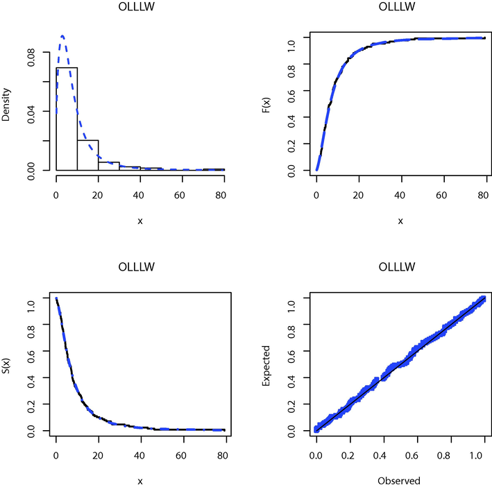
The fitted PDF, CDF, SF and PP plots of the OLLLW model for cancer data.

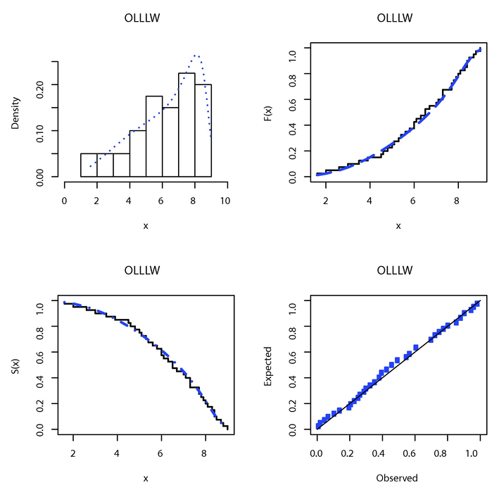
The fitted PDF, CDF, SF and PP plots of the OLLLW model for failure time data.

7 Concluding Remarks

This paper proposed a more flexible extension of the Weibull model called the odd log–logistic Lindley-Weibull (OLLLW) distribution to improve the fitting of the Weibull distribution. The OLLLW density can be expressed as a linear mixture of Weibull densities. The hazard function of the OLLEW provides all important failure rate shapes including bathtub, decreasing, unimodel, increasing, J shaped or reversed-J shaped. Some basic properties are calculated. The parameters of the OLLLW distribution are estimated using some classical estimators including the maximum likelihood, least-squares, Cramér-von Mises, Anderson–Darling and weighted least squares estimators. The simulation results illustrated that the five estimation methods are performing very well for estimating the parameters of the OLLLW model. The importance and flexibility of the OLLLW distribution are studied using two real data sets from medicine and engineering fields. The OLLLW model provides better fit to the analyzed data as compared with other competing models.

Acknowledgments

The author would like to thank the Editorial Board and the reviewers for their valuable suggestions, which improved the current version of the paper.

Declaration of Competing Interest

The authors declare that they have no known competing financial interests or personal relationships that could have appeared to influence the work reported in this paper.

References

Abouelmagd T.H.M., Al-mualim S., Afify A.Z., Ahmad M., Al-Mofleh H., . The odd Lindley Burr XII distribution with applications. Pakistan J. Stat.. 2018;34(1):15-32.
[Google Scholar]
Abouelmagd T.H.M., Al-mualim S., Elgarhy M., Afify A.Z., Ahmad M., . Properties of the four-parameter Weibull distribution and its applications. Pakistan J. Stat.. 2017;33(6):449-466.
[Google Scholar]
Afify A.Z., Alizadeh M., . The odd Dagum family of distributions: properties and applications. J. Appl. Probab. Stat. 2020;15:45-72.
[Google Scholar]
Afify A.Z., Cordeiro G.M., Butt N.S., Ortega E.M.M., Suzuki A.K., . A new lifetime model with variable shapes for the hazard rate. Brazilian J. Prob. Stat.. 2017;31(3):516-541.
[Google Scholar]
Afify A.Z., Alizadeh M., Zayed M., Ramires T.G., Louzada F., . The odd log-logistic exponentiated Weibull distribution: Regression modeling, properties, and applications. Iranian J. Sci. Technol., Trans. A: Sci.. 2018;42(4):2273-2288.
[Google Scholar]
Afify A.Z., Kumar D., Elbatal I., . Marshall-Olkin power generalized Weibull distribution with applications in engineering and medicine. J. Stat. Theory Appl. 2020
[Google Scholar]
Afify A.Z., Nassar M., Cordeiro G.M., Kumar D., . The Weibull Marshall-Olkin Lindley distribution: Properties and estimation. J. Taibah Univ. Sci.. 2020;14(1):192-204.
[Google Scholar]
Afify A.Z., Gemeay A.M., Ibrahim N.A., . The heavy-tailed exponential distribution: Risk measures, estimation, and application to actuarial data. Mathematics. 2020;8:1276.
[Google Scholar]
Ahmad Z., Elgarhy M., Hamedani G.G., . A new Weibull-x family of distributions: properties, characterizations and applications. J. Stat. Distributions Appl.. 2018;5(1):1-18.
[Google Scholar]
Aldahlan M.A., Afify A.Z., . The odd exponentiated half-logistic exponential distribution: estimation methods and application to engineering data. Mathematics. 2020;8(10):1684.
[Google Scholar]
Alizadeh, M., Altun, E., Afify, A.Z., Ozel, G., 2018. The extended odd Weibull-G family: properties and applications. Communications Faculty of Sciences University of Ankara Series A1 Mathematics and Statistics, 68(1), 161–186.
Alizadeh M., Afify A.Z., Eliwa M.S., Ali S., . The odd log-logistic Lindley-g family of distributions: properties, bayesian and non-bayesian estimation with applications. Comput. Statistics. 2020;35(1):281-308.
[Google Scholar]
Alkarni S., Afify A.Z., Elbatal I., Elgarhy M., . The extended inverse Weibull distribution: Properties and applications. Complexity. 2020;2020
[Google Scholar]
Al-Mofleh H., Afify A.Z., Ibrahim N.A., . A new extended two-parameter distribution: Properties, estimation methods, and applications in medicine and geology. Mathematics. 2020;8(9):1578.
[Google Scholar]
Aryal G.R., Tsokos C.P., . Transmuted Weibull distribution: A generalization of the Weibull probability distribution. Eur. J. Pure Appl. Math.. 2011;4(2):89-102.
[Google Scholar]
Bourguignon M., Silva R.B., Cordeiro G.M., . TheWeibull-G family of probability distributions. J. Data Sci.. 2014;12(1):53-68.
[Google Scholar]
Cordeiro G.M., Ortega E.M.M., Nadarajah S., . The Kumaraswamy Weibull distribution with application to failure data. J. Franklin Inst.. 2010;347(8):1399-1429.
[Google Scholar]
Cordeiro, G.M., Afify, A.Z., Yousof, H.M., Pescim, R.R., Aryal, G.R., 2017. The exponentiated Weibull-H family of distributions: Theory and applications. Mediterranean Journal of Mathematics, 14(4):p.155, 2017.
Cordeiro G.M., Afify A.Z., Ortega E.M.M., Suzuki A.K., Mead M.E., . The odd Lomax generator of distributions: Properties, estimation and applications. J. Comput. Appl. Math.. 2019;347:222-237.
[Google Scholar]
Elbatal I., Zayad M., Rasekhi M., Afify A., Iqbal Z., . A new extended Weibull model for lifetime data. J. Appl. Prob. Stat.. 2019;4:57-73.
[Google Scholar]
He W., Ahmad Z., Afify A.Z., Goual H., . The arcsine exponentiated-X family: Validation and insurance application. Complexity. 2020;2020
[Google Scholar]
Korkmaz M., Cordeiro G.M., Yousof H.M., Pescim R.R., Afify A.Z., Nadarajah S., . The Weibull Marshall-Olkin family: Regression model and application to censored data. Commun. Statistics-Theory Methods. 2019;48(16):4171-4194.
[Google Scholar]
Kotz S., Nadarajah S., . Extreme value distributions: theory and applications. World Scientific; 2000.
Lee E.T., Wang J., . Statistical methods for survival data analysis. Vol volume 476. John Wiley & Sons; 2003.
Lee C., Famoye F., Olumolade O., . Beta-Weibull distribution: some properties and applications to censored data. J. Modern Appl. Stat. Methods. 2007;6(1):17.
[Google Scholar]
Marshall A.W., Olkin I., . A new method for adding a parameter to a family of distributions with application to the exponential and weibull families. Biometrika. 1997;84(3):641-652.
[Google Scholar]
Mead M.E., Cordeiro G.M., Afify A.Z., Al Mofleh H., . The alpha power transformation family: properties and applications. Pakistan J. Stat. Operation Res. 2019:525-545.
[Google Scholar]
Mudholkar G.S., Srivastava D.K., . Exponentiated Weibull family for analyzing bathtub failure-rate data. IEEE Trans. Reliab.. 1993;42(2):299-302.
[Google Scholar]
Nassar M., Afify A.Z., Dey S., Kumar D., . A new extension of Weibull distribution: properties and different methods of estimation. J. Comput. Appl. Math.. 2018;336:439-457.
[Google Scholar]
Nassar M., Afify A.Z., Shakhatreh M., Dey S., . On a new extension of Weibull distribution: Properties, estimation, and applications to one and two causes of failures. Qual. Reliab. Eng. Int.. 2020;36(6):2019-2043.
[Google Scholar]
Nassar M., Afify A.Z., Shakhatreh M.K., Dey S., . On a new extension of Weibull distribution: Properties, estimation, and applications to one and two causes of failures. Quality Reliab. Eng. Int.. 2020;36(6):2019-2043.
[Google Scholar]
Peng X., Yan Z., . Estimation and application for a new extended Weibull distribution. Reliab. Eng. System Safety. 2014;121:34-42.
[Google Scholar]
Provost S.B., Saboor A., Ahmad M., . The gamma-Weibull distribution. Pak. J. Statist. 2011;27(2):111-131.
[Google Scholar]
Saboor A., Kamal M., Ahmad M., . The transmuted exponential–Weibull distribution with applications. Pak. J. Statist. 2015;31(2):229-250.
[Google Scholar]
Saboor A., Khan M.N., Cordeiro G.M., Pascoa M.A.R., Bortolini J., Mubeen S., . Modified beta modified-Weibull distribution. Comput. Statistics. 2019;34(1):173-199.
[Google Scholar]
Sen S., Afify A.Z., Al-Mofleh H., Ahsanullah M., . The quasi xgamma-geometric distribution with application in medicine. Filomat. 2019;33(16):5291-5330.
[Google Scholar]
Teamah A.A.M., Elbanna A.A., Gemeay A.M., . Fréchet-Weibull distribution with applications to earthquakes data sets. Pakistan J. Stat.. 2020;36(2)
[Google Scholar]
Xie M., Tang Y., Goh T.N., . A modified Weibull extension with bathtub-shaped failure rate function. Reliab. Eng. System Safety. 2002;76(3):279-285.
[Google Scholar]
Zhang T., Xie M., . On the upper truncated Weibull distribution and its reliability implications. Reliab. Eng. Syst. Safety. 2011;96(1):194-200.
[Google Scholar]
Zichuan M., Hussain S., Iftikhar A., Ilyas M., Ahmad Z., Khan D.M., Manzoor S., . A new extended-family of distributions: Properties and applications. Comput. Math. Methods Med.. 2020;2020
[Google Scholar]

Show Sections

[1] Abouelmagd T.H.M., Al-mualim S., Afify A.Z., Ahmad M., Al-Mofleh H., . The odd Lindley Burr XII distribution with applications. Pakistan J. Stat.. 2018;34(1):15-32.
[Google Scholar]

[2] Abouelmagd T.H.M., Al-mualim S., Elgarhy M., Afify A.Z., Ahmad M., . Properties of the four-parameter Weibull distribution and its applications. Pakistan J. Stat.. 2017;33(6):449-466.
[Google Scholar]

[3] Afify A.Z., Alizadeh M., . The odd Dagum family of distributions: properties and applications. J. Appl. Probab. Stat. 2020;15:45-72.
[Google Scholar]

[4] Afify A.Z., Cordeiro G.M., Butt N.S., Ortega E.M.M., Suzuki A.K., . A new lifetime model with variable shapes for the hazard rate. Brazilian J. Prob. Stat.. 2017;31(3):516-541.
[Google Scholar]

[5] Afify A.Z., Alizadeh M., Zayed M., Ramires T.G., Louzada F., . The odd log-logistic exponentiated Weibull distribution: Regression modeling, properties, and applications. Iranian J. Sci. Technol., Trans. A: Sci.. 2018;42(4):2273-2288.
[Google Scholar]

[6] Afify A.Z., Kumar D., Elbatal I., . Marshall-Olkin power generalized Weibull distribution with applications in engineering and medicine. J. Stat. Theory Appl. 2020
[Google Scholar]

[7] Afify A.Z., Nassar M., Cordeiro G.M., Kumar D., . The Weibull Marshall-Olkin Lindley distribution: Properties and estimation. J. Taibah Univ. Sci.. 2020;14(1):192-204.
[Google Scholar]

[8] Afify A.Z., Gemeay A.M., Ibrahim N.A., . The heavy-tailed exponential distribution: Risk measures, estimation, and application to actuarial data. Mathematics. 2020;8:1276.
[Google Scholar]

[9] Ahmad Z., Elgarhy M., Hamedani G.G., . A new Weibull-x family of distributions: properties, characterizations and applications. J. Stat. Distributions Appl.. 2018;5(1):1-18.
[Google Scholar]

[10] Aldahlan M.A., Afify A.Z., . The odd exponentiated half-logistic exponential distribution: estimation methods and application to engineering data. Mathematics. 2020;8(10):1684.
[Google Scholar]

[11] Alizadeh, M., Altun, E., Afify, A.Z., Ozel, G., 2018. The extended odd Weibull-G family: properties and applications. Communications Faculty of Sciences University of Ankara Series A1 Mathematics and Statistics, 68(1), 161–186.

[12] Alizadeh M., Afify A.Z., Eliwa M.S., Ali S., . The odd log-logistic Lindley-g family of distributions: properties, bayesian and non-bayesian estimation with applications. Comput. Statistics. 2020;35(1):281-308.
[Google Scholar]

[13] Alkarni S., Afify A.Z., Elbatal I., Elgarhy M., . The extended inverse Weibull distribution: Properties and applications. Complexity. 2020;2020
[Google Scholar]

[14] Al-Mofleh H., Afify A.Z., Ibrahim N.A., . A new extended two-parameter distribution: Properties, estimation methods, and applications in medicine and geology. Mathematics. 2020;8(9):1578.
[Google Scholar]

[15] Aryal G.R., Tsokos C.P., . Transmuted Weibull distribution: A generalization of the Weibull probability distribution. Eur. J. Pure Appl. Math.. 2011;4(2):89-102.
[Google Scholar]

[16] Bourguignon M., Silva R.B., Cordeiro G.M., . TheWeibull-G family of probability distributions. J. Data Sci.. 2014;12(1):53-68.
[Google Scholar]

[17] Cordeiro G.M., Ortega E.M.M., Nadarajah S., . The Kumaraswamy Weibull distribution with application to failure data. J. Franklin Inst.. 2010;347(8):1399-1429.
[Google Scholar]

[18] Cordeiro, G.M., Afify, A.Z., Yousof, H.M., Pescim, R.R., Aryal, G.R., 2017. The exponentiated Weibull-H family of distributions: Theory and applications. Mediterranean Journal of Mathematics, 14(4):p.155, 2017.

[19] Cordeiro G.M., Afify A.Z., Ortega E.M.M., Suzuki A.K., Mead M.E., . The odd Lomax generator of distributions: Properties, estimation and applications. J. Comput. Appl. Math.. 2019;347:222-237.
[Google Scholar]

[20] Elbatal I., Zayad M., Rasekhi M., Afify A., Iqbal Z., . A new extended Weibull model for lifetime data. J. Appl. Prob. Stat.. 2019;4:57-73.
[Google Scholar]

[21] He W., Ahmad Z., Afify A.Z., Goual H., . The arcsine exponentiated-X family: Validation and insurance application. Complexity. 2020;2020
[Google Scholar]

[22] Korkmaz M., Cordeiro G.M., Yousof H.M., Pescim R.R., Afify A.Z., Nadarajah S., . The Weibull Marshall-Olkin family: Regression model and application to censored data. Commun. Statistics-Theory Methods. 2019;48(16):4171-4194.
[Google Scholar]

[23] Kotz S., Nadarajah S., . Extreme value distributions: theory and applications. World Scientific; 2000.

[24] Lee E.T., Wang J., . Statistical methods for survival data analysis. Vol volume 476. John Wiley & Sons; 2003.

[25] Lee C., Famoye F., Olumolade O., . Beta-Weibull distribution: some properties and applications to censored data. J. Modern Appl. Stat. Methods. 2007;6(1):17.
[Google Scholar]

[26] Marshall A.W., Olkin I., . A new method for adding a parameter to a family of distributions with application to the exponential and weibull families. Biometrika. 1997;84(3):641-652.
[Google Scholar]

[27] Mead M.E., Cordeiro G.M., Afify A.Z., Al Mofleh H., . The alpha power transformation family: properties and applications. Pakistan J. Stat. Operation Res. 2019:525-545.
[Google Scholar]

[28] Mudholkar G.S., Srivastava D.K., . Exponentiated Weibull family for analyzing bathtub failure-rate data. IEEE Trans. Reliab.. 1993;42(2):299-302.
[Google Scholar]

[29] Nassar M., Afify A.Z., Dey S., Kumar D., . A new extension of Weibull distribution: properties and different methods of estimation. J. Comput. Appl. Math.. 2018;336:439-457.
[Google Scholar]

[30] Nassar M., Afify A.Z., Shakhatreh M., Dey S., . On a new extension of Weibull distribution: Properties, estimation, and applications to one and two causes of failures. Qual. Reliab. Eng. Int.. 2020;36(6):2019-2043.
[Google Scholar]

[31] Nassar M., Afify A.Z., Shakhatreh M.K., Dey S., . On a new extension of Weibull distribution: Properties, estimation, and applications to one and two causes of failures. Quality Reliab. Eng. Int.. 2020;36(6):2019-2043.
[Google Scholar]

[32] Peng X., Yan Z., . Estimation and application for a new extended Weibull distribution. Reliab. Eng. System Safety. 2014;121:34-42.
[Google Scholar]

[33] Provost S.B., Saboor A., Ahmad M., . The gamma-Weibull distribution. Pak. J. Statist. 2011;27(2):111-131.
[Google Scholar]

[34] Saboor A., Kamal M., Ahmad M., . The transmuted exponential–Weibull distribution with applications. Pak. J. Statist. 2015;31(2):229-250.
[Google Scholar]

[35] Saboor A., Khan M.N., Cordeiro G.M., Pascoa M.A.R., Bortolini J., Mubeen S., . Modified beta modified-Weibull distribution. Comput. Statistics. 2019;34(1):173-199.
[Google Scholar]

[36] Sen S., Afify A.Z., Al-Mofleh H., Ahsanullah M., . The quasi xgamma-geometric distribution with application in medicine. Filomat. 2019;33(16):5291-5330.
[Google Scholar]

[37] Teamah A.A.M., Elbanna A.A., Gemeay A.M., . Fréchet-Weibull distribution with applications to earthquakes data sets. Pakistan J. Stat.. 2020;36(2)
[Google Scholar]

[38] Xie M., Tang Y., Goh T.N., . A modified Weibull extension with bathtub-shaped failure rate function. Reliab. Eng. System Safety. 2002;76(3):279-285.
[Google Scholar]

[39] Zhang T., Xie M., . On the upper truncated Weibull distribution and its reliability implications. Reliab. Eng. Syst. Safety. 2011;96(1):194-200.
[Google Scholar]

[40] Zichuan M., Hussain S., Iftikhar A., Ilyas M., Ahmad Z., Khan D.M., Manzoor S., . A new extended-family of distributions: Properties and applications. Comput. Math. Methods Med.. 2020;2020
[Google Scholar]

The extended Weibull distribution with its properties, estimation and modeling skewed data

Abstract

Keywords

Anderson–Darling estimators

Cramér-von Mises estimation

Moments

odd log–logistic Lindley family

Simulation

Weibull distribution

60E05

62F10

1 Introduction

2 The OLLLW distribution

3 Mathematical Properties

3.1 Linear Representation

3.2 Moments

3.3 Incomplete Moments

3.4 Generating Function

3.5 Order Statistics

4 Methods of Estimation

4.1 Maximum Likelihood Estimation

4.2 Ordinary Least-Squares and Weighted Least-Squares Estimators

4.3 Anderson–Darling Estimation

4.4 Cramér–von Mises Estimation

5 Simulation Results

6 Real Data Applications

7 Concluding Remarks

Acknowledgments

Declaration of Competing Interest

References

Suggested read for related articles: