The exact solutions of the $\left(2+1\right)$ –dimensional Kadomtsev–Petviashvili equation with variable coefficients by extended generalized $\left(\frac{G^{\prime }}{G}\right)$ -expansion method

1 Introduction

The study of nonlinear evolution equations and soliton theory is significant for the physical models in different scientific fields such as physics, chemistry, biology, mathematical physics, and plasma physics (Hirota, 2004). The exact solutions of nonlinear partial differential equations plays an important role to understand the dynamical structure of the physical models, to obtain such exact solutions, different types of analytical methods are applied such as generalized exponential rational function method (Kumar, 2021), Lie symmetry approach (Kumar and Niwas, 2021), Kudryashov’s method (Alotaibi, 2021), $\left(\frac{G^{\prime }}{G}\right)$ –expansion method (Mohanty and Dev, 2021), generalized $\left(\frac{G^{\prime }}{G}\right)$ –expansion method (Foroutan et al., 2018; Naher and Abdullah, 2013), generalized and improved $\left(\frac{G^{\prime }}{G}\right)$ –expansion method (Mohanty et al., 2022), extended generalized $\left(\frac{G^{\prime }}{G}\right)$ –expansion method (Mohanty et al., 2021) etc.

Invariance analysis frequently employs equations of higher-dimensional nonlinear development. The dissipative long wave equation (Kumar and Rani, 2021), the Pavlov equation (Kumar and Rani, 2020), the Boussinesq equation (Kumar and Rani, 2021), the Sharma-Tasso-Olver equation (Kumar et al., 2021), the Bogoyvlenskip Scheff equation (Kumar and Rani, 2021), and the Kadomtsev–Petviashvili equation (Rani et al., 2021) are a few examples of these equations. These equations have single soliton, multisoliton, periodic soliton, bright soliton, kink wave soliton, and kink wave type solitons, which have several applications in the solitary wave theory.

Out of these equations, the KP equation exists extensively in studying waves in dynamical system (Groves and Sun, 2008). Further, the KP equation exists in the field of dusty plasma (Seadawy and Rashidy, 2018; Samanta et al., 2013; Saha et al., 2015), in Ocean Engineering (Gwinn, 1997).

sIn this paper, we consider a general form of the $\left(2+1\right)$ -dimensional KP equation with variable coefficients, which is as follows

The symmetry property of the exact solutions of $\left(2+1\right)$ –dimensional KP equation with variable coefficients is studied by Ma et al. (2013) by using a simple direct method. Borhanifar and Abazari (2011), studied the periodic and solitary wave solutions of the generalized $\left(2+1\right)$ –dimensional KP equation with constant coefficients by using the $\left(\frac{G^{\prime }}{G}\right)$ –expansion method. The soliton-like solutions of generalized KP equation with variable coefficients are obtained using the extended hyperbolic function method (Gao, 2001). The breather wave and cross-kink solutions of the $\left(2+1\right)$ –dimensional KP equation with variable coefficients has been studied by Huang et al. (2020). On the other hand, the exact solutions of the KP equation with constant coefficient are obtained by using different methods such as $\exp \left(-\mathrm{\Psi }\left(Z\right)\right)$ –expansion method, and extended complex method (Gu and Meng, 2019), $\left(\frac{G^{\prime }}{G},\frac{1}{G}\right)$ –expansion method (Yang and He, 2013), Lie symmetry analysis (Malik et al., 2021), extended homogeneous balance method (Abdelsalam and Allehiany, 2018).

The extended generalized $\left(\frac{G^{\prime }}{G}\right)$ –expansion method (Mohanty et al., 2021) is a well defined, simple and effective method, which has been already applied to solve the Schamel Burgers and the Schamel equation with constant coefficients (Mohanty et al., 2021). The idea behind the extended generalized expansion method is that, it is based on the initial assumption solution for the nonlinear evolution equation, which can be a represented by the polynomial of $\left(\frac{G^{\prime }}{G}\right)$ , where the coefficients of the polynomial are functions of $\xi$ , and $G=G(\xi )$ satisfies the differential equation of the form

2 The extended $\left(\frac{G^{\prime }}{G}\right)$ expansion method and new exact solutions

Consider the nonlinear partial differential equation of the form

In the extended generalized $\left(\frac{G^{\prime }}{G}\right)$ expansion method the assumed solutions of (3) can be written as polynomial of $\left(\frac{G^{\prime }}{G}\right)$ with degree m, as follows (Mohanty et al., 2021).

The general solution of equation Eq. (2) are given with different conditions in Mohanty et al. (2021), Mohanty et al. (2022), Foroutan et al. (2018), and Naher and Abdullah (2013)

Family-1: When $P_2\ne 0$ and $P_2^2+4P_4\left(P_1-P_3\right)>0$ ,

Family-2: When $P_2\ne 0$ and $P_2^2+4P_4\left(P_1-P_3\right)<0$ ,

Family-3: When $P_2\ne 0$ and $P_2^2+4P_4\left(P_1-P_3\right)=0$ ,

Family-4: When $P_2=0$ and $P_4\left(P_1-P_3\right)>0$ ,

Family-5: When $P_2=0$ and $P_4\left(P_1-P_3\right)>0$ ,

In order to construct the exact solutions with arbitrary functions $\xi (x,y,t)$ for the $\left(2+1\right)$ –dimensional KP Eq. (1), we substitute Eq. (4) into (1). Balancing the highest order derivative term $u_{\mathit{xxxx}}$ with the nonlinear term ${\mathit{uu}}_{\mathit{xx}}$ in (1), we obtained $m=2$ . Thus Eq. (4) can be changed to $$u=b_0(Y)+b_1(Y)\left(\frac{G^{\prime }}{G}\right)+b_2(Y){\left(\frac{G^{\prime }}{G}\right)}^2$$

For simplifying the computation, we choose $b_0(Y)=a(y,t),b_1(Y)=b(y,t),b_2(Y)=c(y,t)$ , and $\xi =p(y,t)+\mathit{kx}$ , where p is function of $y,t$ and k is constant, are to be determined later. Hence the assumed solution of (1) can be written of the form

Now substituting the values of Eq. (10), into Eq. (1), then Eq. (1) is converted in the form of polynomial of $\left(\frac{G^{\prime }}{G}\right)$ of degree 6, then collecting the coefficients of same power of $\left(\frac{G^{\prime }}{G}\right)$ which is equal to zero, we get the system of partial differential equations is a form

New exact solutions of the $\left(2+1\right)$ –dimensional Kadomtsev–Petviashvili Eq. (1) can be obtained as follows. Substituting Eq. (18) and Eq. (5) into Eq. (10), the hyperbolic solution of Eq. (1) is

Substituting Eq. (18) and Eq. (6) into Eq. (10), the trigonometric solution of Eq. (1) is

Substituting Eq. (18) and Eq. (7) into Eq. (10), the rational solution of the Eq. (1) is

Substituting Eq. (18) and Eq. (8) into Eq. (10), the hyperbolic solution of Eq. (1) is

Substituting Eqs. (18) and (9) into equation Eq. (10), Thus the trigonometric solutions of the Eq. (1) is

3 Graphs and discussion

The solutions obtained for the $(2+1)$ –dimensional KP equation with variable coefficients are verified by back substitution in the original equation using the symbolic computational software Mathematica. The graphical representation of some of the obtained solutions are considered by using Mathematica 12. The dynamical structures of the obtained solutions are given as follows Fig. 1–3 illustrates the solitary wave, double soliton, and multisoliton type traveling waves for the KP equation with variable coefficients using the extended generalized expansion method approach through the three-dimensional surface plots and corresponding contour plots. In Fig. 1 the annihilation of surface plot and contour plot of solution (19) represent the solitary type traveling wave soliton, and similar type of dynamic structures of solitary tye wave soliton also exists for solution (22). As seen from Fig. 1 with time, there is a smooth transition of the isolated region which resembles a typical classical solitary wave formation in nonlinear dynamics. Fig. 2 shows a typical formation of double layer type structure for such solution (20). Fig. 2 depicts two types of wave propagation: comprehensive and rarefactive. We know that compressive waveform is where the amplitude is positive, and rarefactive when the amplitude is negative. Fig. 2 shows both positive and negative amplitude, comprising both compressive and rarefactive waveforms. The same double layer structure also exists for the solution (23). Fig. 3 provides the information about the multi-soliton structure of solution (21).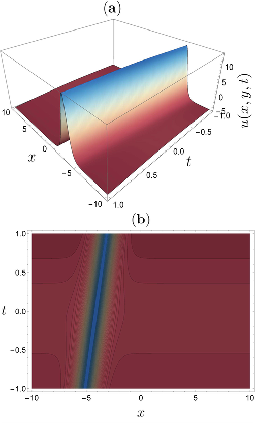

Close

Fig. 1

(a) and (b) are three dimensional surface plot and contour plot of Eq. (19) respectively where the values of the free parameters are taken as $P_1=40,P_2=1,P_3=2,P_4=1,C_1=1,C_2=0,s_1=1,k=8,f(t)=t^2+1,g(t)=t^2+1,h(t)=t^2+1,q_1(t)=t^2+1,f_2(t)=t,f_3(t)=1$ , $y=-8$ , and x varies from $-10$ to $10,t$ varies from $-1$ to 1.

Export to PPT

Close

Fig. 2

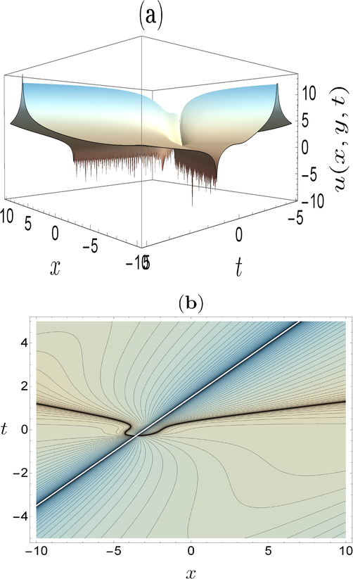
(a) and (b) are three dimensional surface plot and contour plot of from Eq. (20) respectively, where $P_1=30,P_2=10,P_3=2,P_4=-1,C_1=0,C_2=1,s_1=1,k=1,f_2(t)=t,f_3(t)=1,y=-2,f(t)=t^2+1,g(t)=t^2+1,h(t)=t^2+1,q_1(t)=t^2+1$ , and x varies from $-10$ to $10,t$ varies from $-5$ to 5.

Export to PPT

Close

Fig. 3

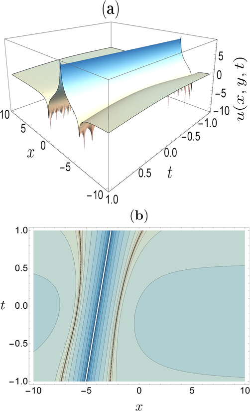
(a) and (b) are three dimensional surface plot and contour plot of Eq. (21) respectively, where $P_1=3,P_2=4,P_3=5,P_4=2,C_1=10,C_2=30,s_1=1,k=5,f_2(t)=t,f_3(t)=1,y=-6,f(t)=t^2+1,g(t)=t^2+1,h(t)=t^2+1,q_1(t)=t^2+1,x$ varies from $-10$ to $10,t$ varies from $-1$ to 1.

Export to PPT

4 Conclusion

The exact solutions of $\left(2+1\right)$ dimensional KP equation with variable coefficients are obtained, for which the extended generalized $\left(\frac{G^{\prime }}{G}\right)$ –expansion method is employed. The resulting solutions are trigonometric, hyperbolic, and rational functions. Dynamical structures of the obtained solutions are the solitary wave, double layer soliton, and multi soliton structures. The graphical representations of the figures also ensure the typical properties of solitonic characteristics of the nonlinear wave dynamics of plasma physics, which is quite encouraging. We believe this method can also be safely applied in nonlinear plasma physics wherein such a situation arises. The method and solutions obtained may help study degenerate nonlinear plasma physics and compact astronomical phenomena such as non-rotating neutron stars (Chabrier et al., 2006), ultra-intense laser-plasma (Eliezer et al., 2005), and optical fibers (Njikue et al., 2018).

References

- Different nonlinear solutions of KP equation in dusty plasmas. Arab. J. Sci. Eng.. 2018;43:399-406.
- [Google Scholar]
- Traveling wave solutions to the nonlinear evolution equation using expansion method and addendum to Kudryashov’s method. Symmetry. 2021;13:2126.
- General solution of generalized -dimensional Kadomtsev–Petviashvili (KP) equation by using –expansion method. Am. J. Comput. Math.. 2011;1:219-225.
- Dense plasma in astrophysics: from giant planets to neutron stars. J. Phys. A: Math. Gen.. 2006;39:4411-4419.
- Effects of Landau quantization on the equations of state in thense laser plasma interactions with strong magnetic fields. Phys. Plasmas. 2005;12:052115
- Solitons in optical metamaterials with anti–cubic law of non–linearity by generalized –expansion method. Optik. 2018;162:86-94.
- On a variable coefficient modified KP equation and a generalized variable coefficient KP equation with computerized symbolic computation. Int. J. Modern Phys. C. 2001;12:819-833.
- Fully localized solitary–wave solutions of the three-dimensional gravity–capillary water wave problem. Arch. Rat. Mech. Anal.. 2008;188:1-91.
- Searching for analytical solutions of the –dimensional KP equation by two different systematic methods. Complexity. 2019;1:9314693.
- Two–dimensional long waves in turbulent flow over a sloping bottom. J. Fluid Mech.. 1997;341:195-223.
- The direct method in soliton theory. Cambridge University Press; 2004.
- One-two and three soliton, periodic and cross-kink solutions to the –D variable coefficient KP equation. Modern Phys. Lett. B. 2020;34:2050045.
- Lump and rogue waves for the variable coefficients Kadomtsev-Petviashvili equation in a fluid. Mod. Phys. Lett. B. 2018;32:1850086.
- Some new families of exact solitary wave solutions of the Klein-Gordon-Zakharov equations in plasma physics. Pramana J. Phys.. 2021;95:161.
- Lie Symmetry Analysis and Dynamics of Exact Solutions of the (2+1))Dimensional Nonlinear Sharma-Tasso-Olver Equation. Math. Prob. Eng.. 2021;9961764
- [CrossRef] [Google Scholar]
- Exact closed-form solutions and dynamics of solitons for a –dimensional universal hierarchy equation via lie approach. Pramana J. Phys.. 2021;95:195.
- Invariance analysis, optimal system, closed-form solutions, and dynamical wave structures of a (2+1))dimensional dissipative long wave system. Phys. Scr.. 2021;96:125202
- Lie symmetry analysis, group-invariant solutions and dynamics of solitons to the (2+1))dimensional Bogoyavlenskii-Schieff equation. Pramana-J. Phys.. 2021;95:51.
- Lie symmetry reductions and dynamics of soliton solutions of (2 + 1))dimensional Pavlov equation. Pramana-J. Phys. 2020;94:116.
- Study of exact analytical solutions and various wave profiles of a new extended (2+1))dimensional Boussinesq equation using symmetry analysis. J. Ocean Eng. Sci. 2021
- Variable–coefficient symbolic computation approach for finding multiple rogue wave solutions of nonlinear system with variable coefficients. Z. Angew. Math. Phys.. 2021;72:154.
- Interaction solutions for Kadomtsev-Petvishvili equation with variable coefficients. Commun. Theor. Phys.. 2019;71:793-797.
- Breather wave solutions for the Kadomtsev-Petviashvili equation with variable coefficients in a fluid based on the variable coefficient three wave approach. Math. Method. Appl. Sci.. 2020;43:458-465.
- Lie symmetry and exact solutions of the –dimensional generalized Kadomtsev-Petviashvili equation with variable coefficients. Therm. Sci.. 2013;17:1490-1493.
- A –dimensional Kadomtsev-Petviashvili equation with competing dispersion effect: Painleve analysis, dynamical behavior and invariant solutions. Results Phys.. 2021;23:104043
- Mohanty, S.K., Dev, A.N., 2021. Study on analytical solutions of KdV equation, Burgers equation, and Schamel KdV equation with different methods. Lecture Notes in Mechanical Engineering, Springer Singapore. pp. 109–136.
- Exact traveling wave solutions of the Schamel Burgers’ equation by using generalized-improved and generalized – expansion methods. Results Phys.. 2022;33:105124
- An efficient technique of -expansion method for modified KdV and Burgers equations with variable coefficients. Results Phys.. 2022;37:105504
- Dynamics of exact closed-form solutions to the Schamel Burgers and Schamel equations with constant coefficients using a novel analytical approach. Int. J. Modern Phys. B. 2021;35:2150317.
- New approach of –expansion method and new approach of generalized –expansion method for nonlinear evolution equation. AIP Adv.. 2013;3:032116
- Exact bright and dark solitary wave solutions of the generalized higher–order nonlinear Schrödinger equation describing the propagation of ultra–short pulse in optical fiber. J. Phys. Commun.. 2018;2:025030
- Invariance analysis for determining the closed-form solutions, optimal system, and various wave profiles for a (2+1))dimensional weakly coupled B-Type Kadomtsev-Petviashvili equations. J. Ocean Eng. Sci. 2021
- Bifurcations and quasi periodic behaviors of ion acoustics waves in magneto plasmas with non thermal electrons featuring tsallis distribution. Braz. J. Phys.. 2015;45:325-333.
- Bifurcations of dust ion acoustic traveling waves in a magnetized dusty plasma with a q-non extensive electron velocity distribution. Phys. Plasmas. 2013;20:022111
- Dispersive solitary wave solutions of Kadomtsev-Petviashvili and modified Kadomtsev-Petviashvili dynamical equations in magnetized dusty plasma. Results Phys.. 2018;8:1216-1222.
- New application of the –expansion method to the KP equation. Appl. Math. Sci.. 2013;7:959-967.
- Wronskian and determinant solutions for a variable coefficient Kadomtsev-Petviashvili equation. Commun. Theor. Phys.. 2008;49:1125-1128.