

Translate this page into:
Surface fitting methods for modelling leaf surface from scanned data
-
Received: ,
Accepted: ,
This article was originally published by Elsevier and was migrated to Scientific Scholar after the change of Publisher.
Peer review under responsibility of King Saud University.
Abstract
Modelling leaves accurately is important in the improvement of a virtual plant model. Therefore an accurate illustration of the leaves are important which can be achieve via mathematical models. These models can be used to study biological procedures for instance, a canopy light environment or photosynthesis. In this research we proposed a new surface fitting method called Gaussion radial basis function Clough-Tocher method (RBF-CT) for modelling a leaf surface. The Gaussion RBF-CT method strategy based on joining the Gaussion radial basis function (RBF) and Clough-Tocher (CT) methods. The accuracy of the presented method is validated by applying it to scattered data taken from Franke (1982) as well as to a real scattered data set collected using a laser scanner from an Anthurium leaf (Loch, 2004). Our method is shown to produces a realistic representation of the leaf surface.
Keywords
Interpolation
Finite elements methods
Virtual leaf
Radial basis function
Clough-Tocher method

1 Introduction
The leaves are vital in the plant development and are essential in any plant model. Our aim in this research is to construct leaf surface model based on scattered data interpolation methods to achieve a continuous surface. The interpolation methods are CT and Gaussion RBF methods.
Modelling of virtual plant has been studied by Anderson (1994), Davydov and Zeilfelder (2004), Espana et al. (1999), Prusinkiewicz (1998), Room et al. (1996), Kempthorne et al. (2015a,b), Dorr et al. (2014), Oqielat et al. (2007, 2011). Loch (2004) sampled data points using laser scanner for Elephant’s ear, Anthurium, Flame and Frangipani leaves and then used finite element method to model the surface of these leaves.
In this paper we reviews the interpolation surface fitting methods based on the RBF and CT techniques. Then, a new hybrid RBF-CT method that combines the CT and Gaussion RBF methods is proposed. Finally, the accuracy of the RBF-CT method is assessed by applying it to a real data points collected using laser scanner from an Anthurium leaf.
The research in this paper is comprises of four main sections. In Section 2, the surface fitting techniques is given. In Section 3, the precision of the methods are evaluated using six test functions and data points chosen from Franke (1982). The quality of the approximation of the methods is measured numerically using the maximum error and the root mean square error. In Section 4, Anthurium leaf surface is constructed using these surface fitting methods. Finally, conclusion and future work is presented in Section 5.
2 Surface fitting techniques
In this section, we will illustrate the RBF, CT and the Gaussion CT-RBF interpolation techniques as well as the application of the methods to two sets of data. The scattered data interpolation problem is given by:
Given
distinct scattered points
, and their function values
, find a function
that interpolates these data satisfying
Finite element methods consist of a triangulation (adopted in this paper) or rectangulation, where the domain is divided into subdomains and then piecewise interpolant is constructed on each element (triangle or rectangle). The value of the function is given at the vertices of the triangle and interpolation polynomial is constructed over each triangle. If the derivatives are not given then they need to be estimated. Finally, by joining the interpolant on each triangle the whole surface is then constructed. For more information see (Lancaster and Salkauskas, 1986).
2.1 The Clough-Tocher method
The Clough-Tocher (CT) method (Clough and Tocher, 1965) is a seamed element method, where each triangle is divide into three micro-elements (subtriangles). A polynomial of degree three is then built on each micro-element to allow a continuous differentiable piecewise cubic polynomial over the whole domain, see (Oqielat et al., 2009, 2007). The form of the CT interpolant is given by:
In this representation the twelve functions
and
are cardinal basis functions (Lancaster and Salkauskas, 1986). To determine
, twelve independent pieces of information are required which consists of the gradient and function values at each vertex as well as the edges normal directional derivative (see Fig. 1). The authors (Turner et al., 2008; Belward et al., 2008) presented analysis for the least square gradient estimation method as well as an error bounds for the method.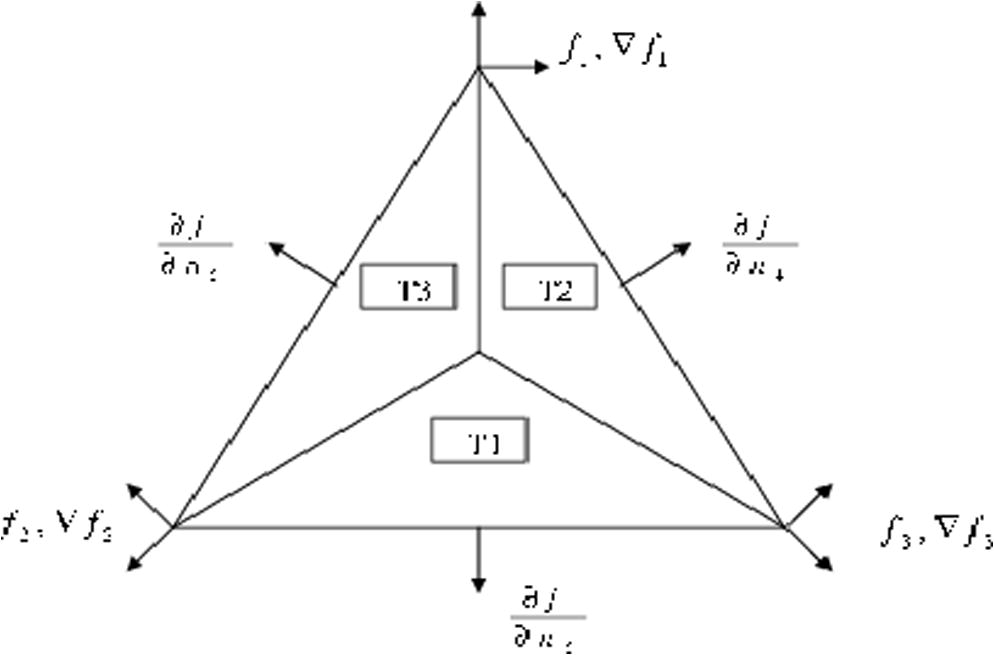
The Triangle of the Clough-Tocher.
2.2 Radial basis functions
The approximation radial basis function
to the function
, is given by:
Radial basis function approach proposes a smooth surface to approximate the values of the function at points. This method has many application in fields for instant, hydrology (Borga and Vizzaccaro, 1997), medical imaging (Carr et al., 1997), geodesy (Junkins et al., 1971), software to drive laser scanners (Carr et al., 2001, 2003), and the partial differential equations solution (Hardy, 1990). Powell (1990) review the theory of RBF.
The computational costs in assessing the RBF to large sets of data points can become time consuming because a large compact matrix system of size
has to be solved in order to calculate the RBF coefficients
in Eq. (4). Franke (1982), compared around 30 interpolation schemes and located that the RBFs are the most accurate methods for surface fitting. Beatson et al. (1999, 2001), Cherrie (2000) used fast evaluation techniques to reduce the computational cost of the RBF. An examples of the RBF comprise thin plate splines, Hardy’s multiquadric (Hardy, 1990) and Gaussian RBF which is adopted in this paper. The Gaussian RBF is given by:
The accuracy of RBF interpolant depends strongly on the parameter where this parameter is specified by the user, see for example (Carlson and Foley, 1991; Niceno, 2003; Sinoquet et al., 1998). For some values of the problem may become ill-conditioned. Franke (1982) and Foley (1987) used where is the diameter of the minimal circle enclosing all data points.
Carlson and Foley (1991) and Franke (1982) studied the accuracy of the multiquadric and inverse multiquadric interpolant and found that the choice of the parameter
has great impact on the accuracy of the RBF. Carlson recurrent the computation of the RMS error with different choices of
and stated the optimal value of
that minimizes the RMS. Rippa (1999) performed experiments on the influence that the parameter
has on the approximation quality achieved using different RBF. Rippa proved that the value of
has impact on the quality of the RBF. Nine test functions and two sets of data are considered by Rippa. He constructed the data vector
by computing each test function over the set of data points so that
An algorithm is proposed by Rippa for the choice of a good value for the parameter that minimizes the RMS error between the RBF interpolant and the unknown function from which the data vector was sampled. The value of is selected by minimizing the cost function. The mnbrak and brent routines from Numerical Recipes [36] were used to do the minimization. The mnbrak routine is given some tolerance and two initial values and . It returns three numbers and that bracket the minimum. After bracketing the minimum, the three numbers and the tolerance parameter are passed into the function brent that uses Brent’s method to minimize the cost function. We refer to the minimum value of the cost function as the “good value” of . The cost function is given by:
Let
be the vector
Rippa showed that
In this research we used another way to minimize the cost function based on using the Matlab command call fminbnd. The Fminbnd return the local minimum of a single-variable function on a fixed interval using either the bisection method twice on the interval or the trisection method which divide the interval into three equal parts. One can see from our numerical result that the value of c obtained using fminbnd are comparable to the values of c obtained using the Rippa method.
2.2.1 The solution of the linear system
The matrix
in (6) is invertible if and only if Eq. (4) has a unique solution. Micchelli (1984) propose conditions on invertibility of
that can be checked for the multiquadric RBF and Gaussion RBF. However, the approximation solution of the linear system is computed by applying the truncated singular value decomposition (TSVD) of
(Tony et al., 1990).
We applied TSVD (Moroney, 2006) to castoff the small singular values regarding to the benchmark where the singular values that are equal to, or less than, the product of the largest singular value with a chosen target
(machine epsilon) are ignored. Thus, if
we ignore
. A new matrix
is then formed with rank
defined by:
2.3 Gaussion radial basis function-Clough-Tocher method
A new radial basis function Clough-Tocher (RBF-CT) method for surface fitting is proposed in this paper. This method is based on using local Gaussion RBF or global Gaussion RBF to evaluate the gradient at the midpoints and the vertices of the Clough-Tocher triangle. The Gaussion RBF is given by:
where
is given in Eq. (5). Then, the gradient of
is given by:
2.3.1 Global and local Gaussion RBF-CT approximations
Our surface fitting method based on choosing a subset of points (the triangles vertices) from the whole data set to produce a surface triangulation. Then the global Gaussion RBF-CT and local Gaussion RBF-CT variants are considered. In the global Gaussion RBF-CT method we constructed a global Gaussion RBF interpolant using these points, subsequently is used to compute the gradients for all CT triangles in the mesh. On the other hand, for the local Gaussion RBF-CT method we used a local subset of size of the points ( or in our numerical experiments) to build a local Gaussion RBF interpolant for each triangle. is then used to compute the CT triangle gradients. Note that we choose these points to be the closest points to each of the edge midpoints and to the vertices of the CT element of interest.
The process that uses this RBF-CT method for the purpose of surface reconstruction is given in the following algorithm:
Algorithm 1: The Gaussion RBF-CT Method for Surface reconstruction
INPUT: data points
Step 1: select a subset of data points for the surface triangulation.
Step 2: compute the RBF linear system (4) Using either a local Gaussion RBF built on each triangle from points OR a global Gaussion RBF from points.
Step 3: use the TSVD approach to estimate the solution of the linear system
Step 4: construct the local or the global gradient using the coefficients of the RBF
Step 5: construct the surface by applying the hybrid method either locally Or globally to obtain the derivatives of the CT interpolant.
Two methods to select the parameter for use in the Gaussion RBF were investigated. The first method based on using the algorithm of Rippa either globally or locally while the second method based on using the Matlab command Fminbnd given in Section 2.2. In the global strategy, a total of points (all points) are used to create one global value of for all CT elements; whereas in the local approach, a total of or points are used to obtain a local estimate of for each CT element.
3 Numerical Investigation for the Franke data set
The mathematical technique given in Section 2 is assessed using numerical experiments presented in this section. To evaluate the accuracy of these methods we used six test functions and two subsets of data taken from Franke (1982). The first subset contains 33 points used to assess the accuracy of the methods by computing the root mean square error (RMS) given in Eq. (19), while the second subset consist of
data points which are used to construct the triangulation of the surface, see Oqielat et al., 2009, 2007).
3.1 Gaussion radial basis function Clough-Tocher method
As mentioned before, the gradients of the CT element are not given, we applied the global Gaussion RBF approach that uses all
data points and the local Gaussion RBF approach that use
or
data points to compute the gradient of the CT triangle for the Franke data. The parameter
in the two cases was approximated either globally using the
data points (Table 3), or locally using a selection of
or
neighbouring points for each CT triangle (Table 4).Tables 2 and 3 show the RMS errors for the six test functions using the global and local RBF-CT method where the parameter c computed using Rippa method. We observe that the RMS errors in both cases are almost as good as the exact values given in Table 1. Moreover, the RMS errors obtained using the global RBF-CT method appear similar to those produced using the local RBF-CT method. The parameter
computed using global method is less computationally costly than using
locally because a new value of
must be calculated each time the local RBF is constructed. Table 3 shows as expected the global values of
were always contained in the local ranges of
given for each of the functions.
Function
Exact Gradient
2.6e−3
2.1e−3
1.4e−4
4.1e−5
2.6e−4
8.7e−5
Another observation from Tables 2 and 3 was that the RMS error produced using the local RBF-CT method constructed with
points was always found to be more accurate than the RMS produced for the surface representation constructed from
points (for both cases whether
is approximated globally or locally). Furthermore, it appears from our numerical experimentation for the Franke data that the local gradient estimates obtained when
using a globally determined value of
would be the most computationally competitive of all of our methods when
is large.
Function
Global RBF-CT
Local RBF-CT
m = 40
m = 20
5.1410
4.1e−3
4.2e−3
6.8e−3
5.3375
4.9e−3
4.6e−3
3.5e−3
3.3918
2.1e−4
2.4e−4
5.7e−4
2.3529
2.1e−4
2.4e−4
2.9e−5
4.3286
2.1e−4
2.5e−4
5.3e−4
1.0750
2.0e−5
5.0e−5
4.6e−5
Function
Local RBF-CT (m = 40)
Local RBF-CT (m = 20)
[2.4813 5.1762]
2.7e−3
[0.5239 6.0677]
4.2e−3
[2.1843 13.0018]
4.4e−3
[0.3399 26.2243]
3.1e−3
[1.382 3.2387]
1.9e−4
[0.3942 3.3897]
4.2e−4
[2.1202 2.3270]
1.9e−4
[1.8912 2.3070]
3.9e−5
[3.6589 4.5927]
2.6e−4
[2.1005 10]
3.3e−4
[0.5724 2.7912]
2.4e−5
[0.2375 0.4812]
2.9e−5
In fact the Gaussion RBF-CT method gives RMS errors quite close to the case where the exact gradient is used (see Table 1). We now carry this finding to the next section and explore the suitability of the Gaussion RBF-CT surface fitting strategy for a real leaf data set.
By profiling the codes in Matlab, we observed for the local and global RBF-CT methods that most of the computational time was spent in solving the gradient RBF problems via the TSVD. In conclusion, we found that the global Gaussion RBF-CT method was the most efficient of all methods tested, followed by the local Gaussion RBF-CT method.
4 Application of the Gaussion RBF-CT method to a leaf data set
A set of points collected from real surface of a leaf are required to be able to reconstruct the leaf surface. To evaluate the accuracy of the Gaussion RBF-CT technique, the Gaussion RBF are used to estimate the gradients of the clough-Tocher triangle for the Anthurium leaf triangular mesh (Loch, 2004). The data of the Anthurium leaf comprises of 4,688 leaf surface points and 79 boundary points, see Fig. 2.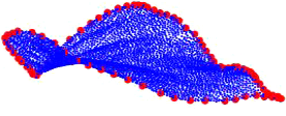
The data points for the Anthurium Leaf. There are 79 boundary points (characterized by the larger dots) and 4,688 surface points (characterized by the smaller dots).
Now to apply the Gaussion RBF-CT method to the Anthurium data, a new reference plane for the data as well as a triangulation for the surface of the leaf are required, see (Oqielat et al., 2009, 2007).
4.1 Reference plane of the leaf data
The leaf data points reference plane may not essential correspond with the -plane in the coordinate system of the data points. To solve this issue a least squares fit to the leaf points is then used as reference plane and then rotating the coordinate system to obtained the -plane as the new reference plane. To achieve the rotations we need at first rotating the reference plane normal vector about the -axis into the -plane and then rotating about the -axis into the -plane, for more details about this procedure, see Oqielat et al. (2007, 2009).
4.2 Leaf surface triangulation
A subset of the Anthurium leaf data set ( points) is selected to reduce the computational cost for surface fitting, these subset are used to generate a triangulation of the surface of the leaf using software written in the C language by Niceno (2003) called EasyMesh mesh generator. EasyMesh produce two-dimensional Delaunay and constrained Delaunay triangulations in general domains. If the domain is convex then a better quality triangulation can be achieved. EasyMesh was not capable to create the wanted triangulation because the 79 Anthurium leaf boundary points do not represent a convex set. To solve this issue we employed an algorithm (Sedgewick, 1988) to produce the convex hull, this algorithm return 49 points. After that, the closest points to these 49 points from the original 79 boundary points were then found using dsearch which is Matlab command. As a result of this process the convex domain shown in Fig. 4(a) is defined using 38 boundary points.
To facilitate EasyMesh to construct fewer and better formed triangles we can define either a vertical line or horizontal or in the inner of the convex hull. Its appear that the vertical line produced a more appropriate triangulation for the Anthurium leaf.
The following steps are applied to generate the triangulation of the Anthurium leaf using EasyMesh:
Step 1: An input file that consists of the vertical line description, the 38 boundary points and the length of the triangle edge for the mesh elements is provided to the EasyMesh. A node file that contained an extra 28 boundary points (introduced during the meshing process) to the original boundary points is return from Easymesh in addition to 146 internal points (vertices of the mesh) distributed inside the leaf shown in Fig. 4(a).
Step 2: We imported the node file that we got in step 2 into Matlab and then the closest points in the leaf data set were located from the internal points generated in step 1 using dsearch. These resulting points were used as the triangle vertices of the leaf surface mesh structure.
Step 3: The surface values of the nearest points from the leaf data points to the EasyMesh boundary points are used as the boundary points of the leaf for which we do not have surface values.
Step 4: The leaf data points that were got from steps 2 and 3 are then used to construct the surface triangulation using the Matlab command delaunay. These four steps produce the final triangulation for the leaf surface shown in Fig. 4(b).
After we generated the triangulation of the Anthurium leaf surface, we applied the local and global Gaussion RBF-CT methods to generate the leaf surface where the gradients at the triangles edge midpoints and the vertices are approximated using the Gaussion RBF (shown in Fig. 3). The global RBF-CT approach based on using the triangulation points to built one global Gaussion RBF and then using it to compute the gradients at the midpoints and vertices of whole triangles in the leaf surface. The local Gaussion RBF-CT approach is based on selecting the closest 30 points to the triangle center and to each of the triangle vertices and then built one local Gaussion RBF from the 120 points on each triangle. This local Gaussion RBF is then used to estimate the gradient at the midpoints and vertices of the CT triangle. In both cases we used Rippa method (Rippa, 1999) to estimate the parameter
globally using the triangular mesh points. The Numerical results for these methods are given in Table 4.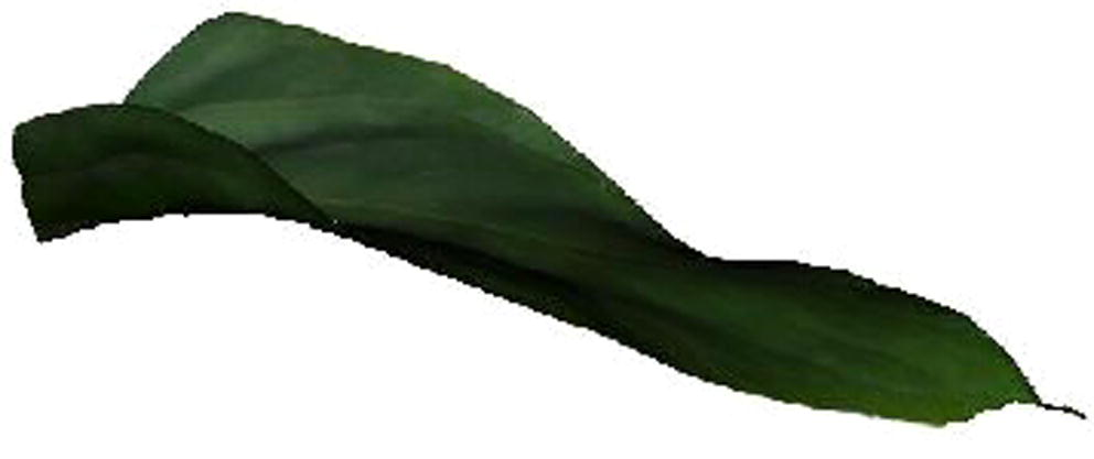
The Anthurium leaf model constructed from the points (shown in Fig. 2) using the Gaussion RBF-CT technique.
Local RBF-CT
Global RBF-CT
RMS Error
0.03234
0.0194
Max. Error
0.9260
0.1206
Triangles Number
178
178
RMS Error
0.1177
0.0098
Max. Error
0.0810
0.0472
Triangles Number
391
391
RMS Error
0.0086
0.0079
Max. Error
0.5331
0.4560
Triangles Number
1486
1486
4.3 Leaf surface numerical experiments
The outcome of applying the Gaussion RBF-CT technique to the data of the Anthurium leaf is given in this section. As mentioned before a subset of the leaf surface data are used for triangulation purposes, the remaining data points of the leaf data (say ) were used to assess the method quality by two error metrics. These two error metrics are the RMS error (see Eq. (19)) and the maximum error associated with the surface fit in relation to the maximum variation in z as where and are respectively the given values of the function and the CT estimated values at the data points ( ).
To achieve a high accurate representation of the leaf surface and to confirm that our results were consistent as the mesh was refined, we used EasyMesh to construct three different triangulation (178, 391 and 1,486 triangles) given in Figs. 4(b) and 5(a)-(b).
Table 4 shows the maximum errors and the relative RMS using the local and global Gaussion RBF-CT techniques for the Anthurium leaf for three different triangulations, see Figs. 4 and 5. The relative RMS was calculated using:
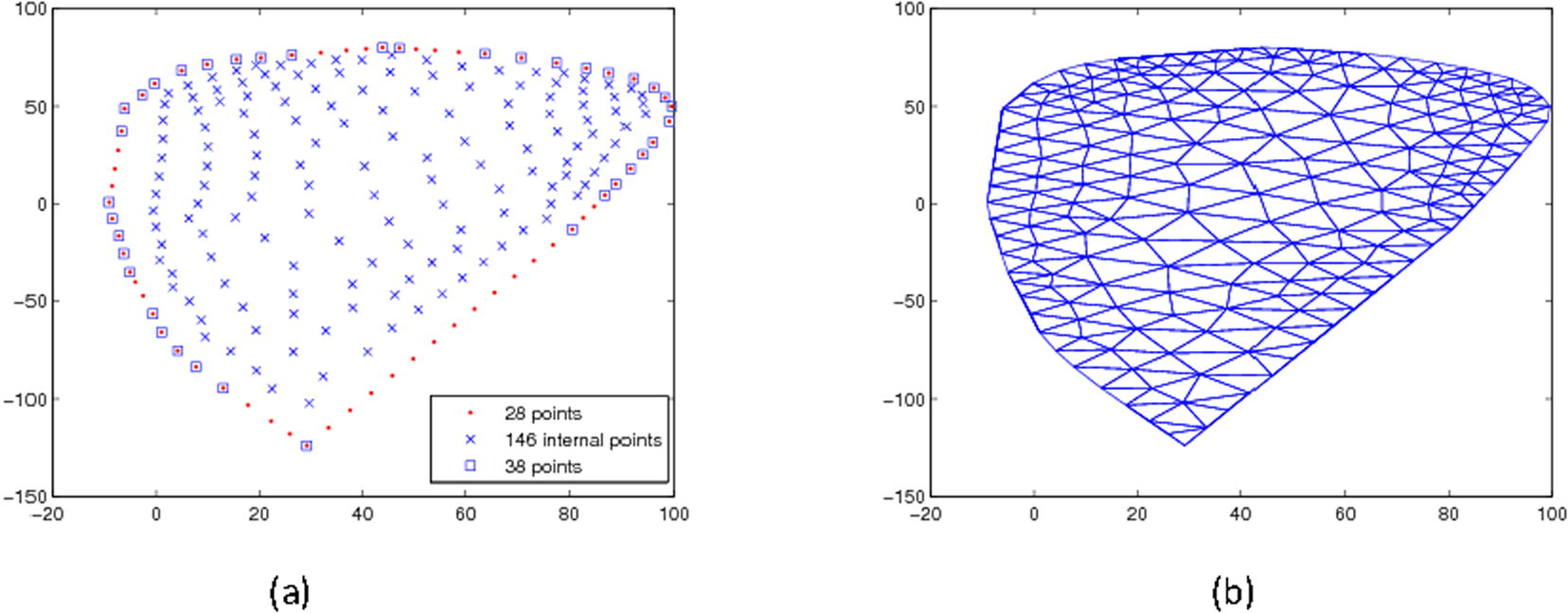
a) The interior (Triangle vertices) and boundary points of the mesh build by Easymesh. The × points are the 146 internal points; the dot points are the 28 extra points added by Easymesh, while The square points are the 38 boundary points that are given to Easymesh. b) Triangulation of the 212 points of the Anthurium leaf surface constructed by EasyMesh.
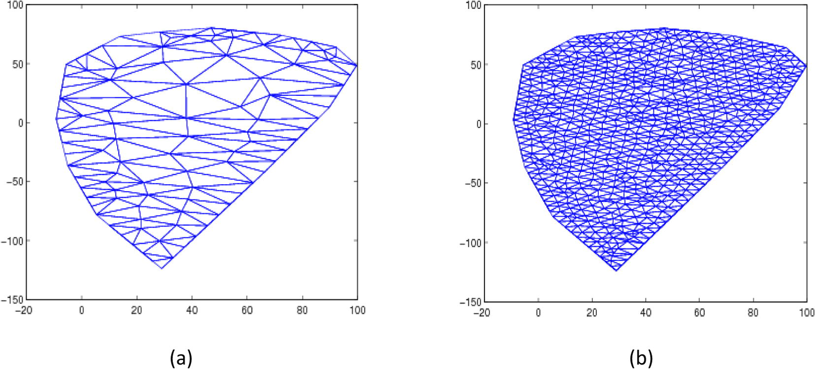
The triangulation of the Anthurium leaf surface constructed using EasyMesh of (a) Rougher mesh of 103 points and (b) a improved mesh of 762 points.
Note that three sets of the Anthurium leaf points were employ to measure the accuracy of the leaf surface. The first set consist of 4,427 data points where the EasyMesh triangulations contained 103 vertices (178 triangles) including 52 boundary points; While the second set consist of 4,460 data points where the EasyMesh triangulations contained 212 vertices (391 triangles) including 66 boundary points; whereas the third set consist of 3,793 data points and the EasyMesh triangulations contained 762 vertices (1486 triangles) including 106 boundary points.
We observed from Table 4 that using the global Gaussion RBF-CT method gave more accurate maximum errors and RMS values than using the local Gaussion RBF-CT method in all three cases. Moreover, a more accurate representation of the surface is obtained for the global method when the number of triangular elements increases. This observation is expected and provides a reasonable justification for the Gaussion RBF-CT method for achieving the leaf surface representation.
The number of points used to build the local Gaussion RBF is important for the gradients estimate accuracy. In our research we have used the closest 30 points to the centroid of the triangle and to each vertex where the computational cost is reasonable and we got the best result, whereas using more points increase the computational expense and does not improve the accuracy much. Moreover using less points result in decreasing the precision of the fit because of inadequate points being employed to deliver a accurate local surface representation to guarantee esensible estimation of the gradient.
5 Conclusions
In this research, we presented a surface fitting method based on mathematics for modelling the surface of the leaf from three-dimensional scanned data points and shown that our method produce an accurate leaf surface representation. The surface representation can be used to find the path of pesticide or water droplet on a leaf surface and then to determine the effectiveness of treatment of different pesticide formulations.
References
- A grid generation and flow solution method for the Euler equations on unstructured grids. J. Comput. Phys.. 1994;110:23-38.
- [Google Scholar]
- Fast fitting of c basis functions: methods based on preconditioned GMRES iteration. Adv. Comput. Math.. 1999;11:253-270.
- [Google Scholar]
- Fast evaluation of radial basis functions: methods for four-dimensional polyharmonic splines. SIAM J. Math. Anal.. 2001;32(6):1272-1310.
- [Google Scholar]
- Belward, J., Turner, I., Oqielat, M., 2008. Numerical Investigation of Linear Least Square Methods for Derivatives Estimation. CTAC 08 Computational Techniques and applications conference, Australia, July 2008.
- On the interpolation of hydrologic variables: formal equivalence of multiquadric surface fitting and kriging. J. Hydrol.. 1997;195:160-171.
- [Google Scholar]
- The parameter R2 in multiquadric interpolation. Comput. Math. Appl.. 1991;21:29-42.
- [Google Scholar]
- Surface interpolation with radial basis functions for medical imaging. IEEE Trans. Med. Imaging. 1997;16(1):96-107.
- [Google Scholar]
- Carr, J.C., Beatson, R.K., Cherrie, J.B., Mitchell, T.J., Fright, W.R., McCallum, B.C., Evans, T.J., 2001. Reconstruction and Representation of 3D Objects with Radial Basis Functions. ACM SIGGRAPH, 12–17 August 2001, Los Angeles, CA, pp. 67–76.
- Carr, J.C., Beatson, R.K., McCallum, B.C., Fright, W.R., McLennan, T.J., Mitchell, T.J., 2003. Smooth surface reconstruction from noisy range data. In: ACM Graphite2003, 11–14 February 2003, Melbourne, Australia, pp. 119–126.
- Fast Evaluation of Radial Basis Functions: Theory and application. New Zealand: University of Canterbury; 2000. (Ph.D. thesis)
- Clough, R.W., Tocher, J.L., 1965. Finite element stiffness matrices for analysis of plate bending. In: Proceedings of the Conference on Matrix Methods in Structural Mechanics. Wright-Patterson A.F.B., Ohio, pp. 515–545.
- Scattered data fitting by direct extension of local polynomials to bivariate splines. Adv. Comput. Math.. 2004;21(3–4):223-271.
- [Google Scholar]
- Towards a model of spray–canopy interactions: interception, shatter, bounce and retention of Droplets on horizontal leaves. Ecol. Model.. 2014;290:94-101.
- [CrossRef] [Google Scholar]
- Radiative transfer sensitivity to the accuracy of canopy structure description. the case of a maize canopy. Agronomie. 1999;19:241-254.
- [Google Scholar]
- Interpolation and approximation of 3-D and 4-D scattered data. Comput. Math. Appl.. 1987;13:711-740.
- [Google Scholar]
- Theory and applications of the multiquadric-biharmonic method. Comput. Math. Appl.. 1990;19:163-208.
- [Google Scholar]
- A weighting function approach to modeling of irregular surfaces. J. Geophys. Res.. 1971;78:1794-1803.
- [Google Scholar]
- Surface reconstruction of wheat leaf morphology from three-dimensional scanned data. Funct. Plant Biol.. 2015;42:444-451. (10.1071/ FP14058)
- [Google Scholar]
- A comparison of techniques for the reconstruction of leaf surfaces from scanned data. SIAM J. Sci. 2015
- [Google Scholar]
- Curve and Surface Fitting, An Introduction. San Diego: Academic Press; 1986.
- Surface Fitting for the Modelling of Plant Leaves. University of Queensland; 2004. (Ph.D. thesis)
- Interpolation of scattered data: distance matrices and conditionally positive definite functions. Constr. Approx.. 1984;2:11-22.
- [Google Scholar]
- Moroney, T., 2006. An Investigation of a Finite Volume Method Incorporating Radial Basis Functions for Simulating Nonlinear Transport (Ph.D. Thesis), Australia, <http://www.sci.qut.edu.au/about/staff/mathsci/computational/moroneyt.jsp>.
- Niceno, B., 2003. Easymesh. <http://www-dinma.univ.trieste.it/nirftc/research/easymesh>.
- Oqielat, M., Belward, J.A., Turner, I.W., Loch, B.I., 2007. A hybrid Clough-Tocher radial basis function method for modelling leaf surfaces. In: MODSIM 2007 International Congress on Modelling and Simulation. Modelling and Simulation Society of Australia and New Zealand, pp. 400–406.
- A hybrid clough-tocher method for surface fitting with application to leaf data. Appl. Math. Model.. 2009;33:2582-2595.
- [Google Scholar]
- Modelling water droplet movements on a leaf surface. Math. Comput. Simul.. 2011;81:1553-1571.
- [CrossRef] [Google Scholar]
- The Theory of Radial Basis Function Approximation in 1990. Advances in Numerical Analysis, Wavelets, Subdivision Algorithms and Radial Functions. W. Light; 1990.
- Modelling of spatial structure and development of plants: a review. Sci. Hortic.. 1998;74:113-149.
- [Google Scholar]
- An algorithm for selecting a good value for the parameter c in radial basis function interpolation. Adv. Comput. Math.. 1999;11:193-210.
- [Google Scholar]
- Virtual plants: new perspectives for ecologists, pathologists and agricultural scientist. Trends Plant Sci.. 1996;1(1):33-38.
- [Google Scholar]
- Algorithms (second ed.). Reading, Mass: Addison-Wesley; 1988.
- Characterization of the light environment in canopies using 3D digitising and image processing. Ann. Bot.. 1998;82:203-212.
- [Google Scholar]
- Computing truncated singular value decomposition least squares solutions by rank revealing qr-factorizations. SIAM J. Sci. Stat. Comput.. 1990;11(3):519-530.
- [Google Scholar]


