Structure of analytical and numerical wave solutions for the Ito integro-differential equation arising in shallow water waves

1 Introduction

Nonlinear evolution equations are commonly used to model and analyse most natural events. In particular, these equations play an essential role in describing and explaining some sophisticated phenomena arising in heat transfer, wave propagation, fluid dynamics, optics, elasticity, fibres, plasma physics, electrodynamics, biology, chemistry, ocean engineering, condensed matter physics and many other branches in nonlinear science(Helal and Seadawy, 2012; Khater et al., 2001; Khater et al., 2003; Khater et al., 2006; Calin Itu et al., 2019; Vlase et al., 2019; Praveen Agarwal, 2021; Agarwal et al., 2020; Rahmoune et al., 2020; Agarwal et al., 2020). The travelling wave solutions of such equations are utilized to clarify and interpret the physical mechanism in the real life. Consequently, there has been a great interest in the investigation of exact travelling wave solutions (Inc et al., 2020; Iqbal et al., 2018; Helal et al., 2014; Ozkan, 2020; Ahmad et al., 2020). Some scientists have devoted considerable effort to develop various approaches by which one can straightforwardly extract the exact travelling wave solutions for some partial differential equations. Among these approaches, we specify and state the following: the projective Riccati equation approach (Conte and Musette, 1992), the sine–cosine approach (Wazwaz, 2005; Wazwaz, 2004), the tanh-sech principal (Malflieta and Hereman, 1996; Wazwaz, 2004), the $\mathit{exp}(-f(\zeta ))$ -expansion process (Alharbi and Almatrafi, 2020), the Adomian decomposition technique (Adomain, 1994; Wazwaz, 2002), the complex hyperbolic function approach (Zayed et al., 2006; Chow, 1995), the rank analysis process (Feng, 2000), the extended tanh method (Fan, 2000; Wazwaz, 2007). For more information about other techniques, one can see Cesar and Gomez (2010), Alharbi et al. (2019), Alharbi and Almatrafi (2020), Alharbi and Almatrafi (2020), Abdelrahman et al. (2020), Alharbi et al. (2020), Alharbi et al. (2020), Alam and Tunç (2019), Shahida and Tunç (2019), Seadawy et al. (2019).

The $(1+1)$ -dimensional Ito equation which is given by

The construction of the exact solutions of Eq. (1) is remarkably limited to some approaches. Thus, we invoke the improved F-expansion process combined with Riccati equation to construct some exact travelling wave solutions for this equation. According to Islam et al. (2014), this method leads to more novel exact travelling wave solutions. The main strategy depends on reducing the integro-differential equation into an appropriate ordinary differential equation (ODE) solved by the considered method. Naturally, the achieved ODE does not provide the whole solutions of the considered PDE, but gives a class of solutions under some conditions. Since the traditional approaches cannot be sometimes applied to handle most nonlinear PDEs, we exploit the numerical methods to approximate the solutions. The finite difference formulae are executed to develop the numerical solutions of Ito equation. The exact and numerical solutions are found nearly the same in the behaviour with a very small error, as can be seen in the presented figures and the provided table.

2 Analysis of the improved F-expansion approach

In this section, we introduce and explain the analysis of the improved F-expansion technique combined with Riccati equation, as presented in Islam et al. (2014). Consider the Riccati equation on the form:

• If $r<0$ , the general solutions of Eq. (2) are formed as

  (3)
  $$F=-\sqrt{-r}\mathit{tanh}(\sqrt{-r}\zeta ),$$
  (4)
  $$F=-\sqrt{-r}\mathit{coth}(\sqrt{-r}\zeta )\text{.}$$

• If $r=0$ , the general solutions of Eq. (2) are expressed as

  (5)
  $$F=-\frac{1}{\zeta }\text{.}$$

• If $r>0$ , the general solutions of Eq. (2) become

  (6)
  $$F=\sqrt{r}\mathit{tan}(\sqrt{r}\zeta ),$$
  (7)
  $$F=-\sqrt{r}\mathit{cot}(\sqrt{r}\zeta )\text{.}$$

Now, we consider the following PDE:

3 Establishment of exact solutions

In this part, we derive new hyperbolic and trigonometric travelling wave solutions for the following equations:

The transform

Integrating twice w.r.t. $\zeta$ and equating the integral constants to zero lead to

The homogeneous balance between ${\mathrm{\Psi }}_{\zeta \zeta \zeta }$ and ${\mathrm{\Psi }}_{\zeta }^2$ gives $M=1$ . Therefore, the travelling wave solution becomes

Next, we plug Eq. (17) into Eq. (16) and equate the coefficients of $F^n,n=0,1,2,\dots ,8$ , to zero to obtain an algebraic system whose solutions are given by

Here, $v_{i,j}$ and $V_{i,j}$ are the exact solutions of Eqs. (13) and (12), respectively. The index i indicates the solution number while j illustrates the case number. Hence, the exact solutions of Eqs. (13) and (12) can be simply formed as follows:

1. If $r<0\mathrm{and}k=-1$ . We have

   Case 1:

   (19)
   $$v_{1,1}(x,t)={\gamma }_0+\frac{6\left(k^2{m}^2+k^{2}r\right)}{\beta }{\left(m+\sqrt{-r}\mathit{tanh}(\sqrt{-r}(\mathit{kx}+4r{k}^{3}t))\right)}^{-1}\text{.}$$

   Hence, the exact solution of Eq. (12), which is determined by taking the first derivative of $v_{1,1}$ with respect to x, is

   (20)
   $$V_{1,1}(x,t)=\frac{6\mathit{kr}\left(k^2{m}^2+k^{2}r\right){\mathit{sech}}^2\left(\sqrt{-r}\left(4k^3\mathit{rt}+\mathit{kx}\right)\right)}{\beta {\left(\sqrt{-r}\tanh \left(\sqrt{-r}\left(4k^3\mathit{rt}+\mathit{kx}\right)\right)+m\right)}^2}\text{.}$$

   Case 2:

   (21)
   $$v_{1,2}(x,t)={\gamma }_0-\frac{6k^{2}r}{\beta }{\left(m+\sqrt{-r}\mathit{tanh}(\sqrt{-r}(\mathit{kx}+4r{k}^{3}t))\right)}^{-1}\text{.}$$

   Therefore, the exact solution of Eq. (12) obtaining by taking the first derivative of $v_{1,2}$ with respect to x, is

   (22)
   $$\begin{array}{c}{V}_{1,2}(x,t)=\frac{6k^3{r}^2{\mathit{sech}}^2\left(\sqrt{-r}\left(4k^3\mathit{rt}+\mathit{kx}\right)\right)}{\beta {\left(\sqrt{-r}\tanh \left(\sqrt{-r}\left(4k^3\mathit{rt}+\mathit{kx}\right)\right)+m\right)}^2}\text{.}\hfill \end{array}$$

   Case 3:

   (23)
   $$v_{1,3}(x,t)={\gamma }_0-\frac{6k^2}{\beta }\left(m+\sqrt{-r}\mathit{tanh}(\sqrt{-r}(\mathit{kx}+4k^{3}rt))\right)\text{.}$$

   Thus, the exact solution of Eq. (12) is shown as follows:

   (24)
   $$\begin{array}{c}{V}_{1,3}(x,t)=\frac{6k^3{\mathit{rsech}}^2\left(\sqrt{-r}\left(4k^3\mathit{rt}+\mathit{kx}\right)\right)}{\beta }\text{.}\hfill \end{array}$$

   Case 4:

   (25)
   $$v_{1,4}(x,t)={\gamma }_0-\frac{6k^2}{\beta }\left(\sqrt{-r}\mathit{tanh}(\sqrt{-r}(\mathit{kx}+16k^{3}rt))\right)+\frac{6k^{2}r}{\beta \left(\sqrt{-r}\mathit{tanh}(\sqrt{-r}(\mathit{kx}+16k^{3}rt))\right)}\text{.}$$

   Hence, the exact solution of Eq. (12) is expressed as

   (26)
   $$V_{1,4}(x,t)=\frac{6r{\mathrm{csch}}^2\left(\sqrt{-r}(-16\mathit{rt}-x)\right)}{\beta }-\frac{6r{\mathrm{sech}}^2\left(\sqrt{-r}(-16\mathit{rt}-x)\right)}{\beta }\text{.}$$

2. If $r>0,k=+1$ then

   Case 1:

   (27)
   $$v_{2,1}(x,t)={\gamma }_0+\frac{6\left(k^2{m}^2+k^{2}r\right)}{\beta }{\left(m+\sqrt{r}\mathit{tan}(\sqrt{r}(\mathit{kx}+4r{k}^{3}t))\right)}^{-1}\text{.}$$

   Thus, the exact solution of Eq. (12) is given by

   (28)
   $$V_{2,1}(x,t)=-\frac{6r\left(m^2+r\right){\sec }^2\left(\sqrt{r}(4\mathit{rt}+x)\right)}{\beta {\left(m+\sqrt{r}\tan \left(\sqrt{r}(4\mathit{rt}+x)\right)\right)}^2}\text{.}$$

   Case 2:

   (29)
   $$v_{2,2}(x,t)={\gamma }_0+\frac{6k^{2}r}{\beta }{\left(\sqrt{r}\mathit{tan}(\sqrt{r}(\mathit{kx}+4r{k}^{3}t))\right)}^{-1}\text{.}$$

   Therefore, the exact solution of Eq. (12) is shown as follows:

   (30)
   $$V_{2,2}(x,t)=-\frac{6r{\csc }^2\left(\sqrt{r}(4\mathit{rt}+x)\right)}{\beta }\text{.}$$

   Case 3:

   (31)
   $$v_{2,3}(x,t)={\gamma }_0-\frac{6k^2}{\beta }\left(m+\sqrt{r}\mathit{tan}(\sqrt{r}(\mathit{kx}+4r{k}^{3}t))\right)\text{.}$$

   Hence, the exact solution of Eq. (12) is given by

   (32)
   $$V_{2,3}(x,t)=-\frac{6r{\sec }^2\left(\sqrt{r}(4\mathit{rt}+x)\right)}{\beta }\text{.}$$

   Case 4:

   (33)
   $$v_{2,4}(x,t)={\gamma }_0-\frac{6k^2}{\beta }\left(\sqrt{r}\mathit{tan}(\sqrt{r}(\mathit{kx}+16r{k}^{3}t))\right)+\frac{6k^{2}r}{\beta \left(\sqrt{r}\mathit{tan}(\sqrt{r}(\mathit{kx}+16r{k}^{3}t))\right)}\text{.}$$

   Thus, the exact solution of Eq. (12) is illustrated as

   (34)
   $$V_{2,4}(x,t)=-\frac{6r{\csc }^2\left(\sqrt{r}(16\mathit{rt}+x)\right)}{\beta }-\frac{6r{\sec }^2\left(\sqrt{r}(16\mathit{rt}+x)\right)}{\beta }\text{.}$$

4 Establishment of numerical solutions

This section is devoted to utterly demonstrate the numerical results of Eqs. (12) and (13) by executing the central finite differences. The numerical solutions are investigated on the interval $[a,b]$ , as illustrated in Fig. 1. Here, a and b denote the endpoints of the physical domain. We begin with generating the numerical solutions of Eq. (13) by reforming Eq. (13) into the following system:

Close

Fig. 1

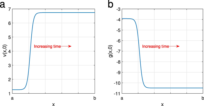
(a) and (b) represent the initial conditions for v and g, respectively, using Eqs. (40). The parameter values are taken by ${\gamma }_0=-2,r=-0.3,\beta =1.2,m=1.2$ .

Export to PPT

The variables x and t indicate the spatial and time variables, respectively. Modifying Eq. (13) into a system leads a scheme much faster and more stable. Let $U=g_{\mathit{xx}}$ . Then, system (35) becomes

The initial conditions of system (37) is generated by introducing the function g which reads

Eq. (19) is selected to build the initial condition of v. Hence, Eq. (38) becomes

Thus, the initial conditions of system (37) are shown as

It is worth noting that Fig. 1 is perfectly utilized to deduce the relevant boundary conditions which are

Here, $\mathrm{\Delta }x$ indicates the space increment. It is important to mention that the numerical results at the mesh node are characterized by $v_n$ and $g_n$ . In addition, we semi-discretize the spatial derivatives whereas the temporal derivatives are kept continuous. Consequently, the new system is given by

The discretization of the term ${\left.g_{\mathit{xxx}}\right|}_n$ and the term ${\left.{\left(v{g}_x\right)}_x\right|}_n$ can be expressed as $$\begin{array}{c}{\left.g_{\mathit{xxx}}\right|}_n=\frac{g_{n+2}-3g_{n+1}+3g_n-g_{n-1}}{2\mathrm{\Delta }{x}^3},\hfill \\ {\left.{\left(v{g}_x\right)}_x\right|}_n=\frac{\left(v_{n+1}+v_n\right)\left(g_{n+1}-g_n\right)-\left(v_n+v_{n-1}\right)\left(g_n-g_{n-1}\right)}{2\mathrm{\Delta }{x}^2}\text{.}\hfill \end{array}$$

The conditions (41) are upgraded with their ODE form

Here, $\mathrm{\Delta }x=(b-a)/N$ . It is to noted that the method of lines is applied here. This approach depends on DASPK solver (Brown et al., 1994) which employs backward differentiation formulas so as to roughly specify time derivatives. Furthermore, the Jacobian matrix of the linearised system is approximated using LU factorization. In order to achieve less bandwidth for the matrix, a unique system numbering for the variables $v_1,g_1,v_2,g_2,\dots ,v_{N-1},g_{N-1},v_N,g_N,v_{N+1},g_{N+1}$ , is used.

5 Result and discussion

In this paper, we have precisely deduced novel exact travelling wave solutions on the form of hyperbolic and trigonometric functions for Eqs. (12) and (13) using the improved F-expansion process combined with Riccati equation. The presented solutions are more general than the solutions investigated by Gepreel et al. (2017) and by Akbari (2017). Akbari (2017) determined one rational solution for the generalized Ito integro-differential equation via the Kudryashov method whereas the authors in Gepreel et al. (2017) applied the generalized Kudryashov technique to extract three rational solutions. The finite difference formulae are perfectly employed in this paper. The achieved numerical solutions are super acceptable. Therefore, the applied methods are more reliable and powerful.

The central finite differences have accurately presented approximated solutions. For instance, Fig. 2 shows that the exact travelling wave solution and the numerical solution of $v(x,t)$ are almost coincident and concomitant. Furthermore, the 2D diagram in Fig. 7 illustrates that the performance of the numerical method for different values of $\mathrm{\Delta }x$ where the smallest value is the best. In particular, when we take $\mathrm{\Delta }x=0.1$ , the resulting $L_2$ error of the numerical solution (dashed yellow line) is large while this error is strongly reduced when we use $\mathrm{\Delta }x=0.001$ , (dashed blue line). Note that all figures are plotted under the values ${\gamma }_0=-2,r=-0.3,\beta =1.2,m=1.2$ . $L_2$ error and CPU time can be easily observed in Table 1. We begin with $\mathrm{\Delta }x=1.000e-01$ where the $L_2$ error reaches $3.206e-01$ in $7.26\times {10}^{-3}$ second. This error arrives at $1.730e-03$ for smaller $\mathrm{\Delta }x=5.000e-03$ during $1.40\times {10}^{-1}$ seconds which increases. However, the method gives suitable performance and shrinks the error for small $\mathrm{\Delta }x=1.000e-03$ with a slight increment in the CPU time ( $6.80\times {10}^{-1}$ s) (see Figs. 3–6).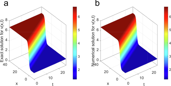

Close

Fig. 2

Graphical comparison between the analytical solution of $v(x,t)$ (left) and the numerical solution of $v(x,t)$ (right). The values of the used parameters are ${\gamma }_0=-2,r=-0.3,\beta =1.2,m=1.2$ .

Export to PPT

Close

Fig. 7

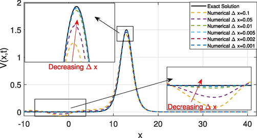
Comparison between the exact and numerical solutions of $V(x,t)$ for various values of $\mathrm{\Delta }x$ . The numerical solution approaches the exact solution if $\mathrm{\Delta }x$ is very small.

Export to PPT

Close

Fig. 3

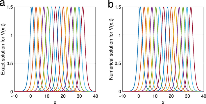
Graphs (a) and (b) represent the time evolution of a single travelling wave for the exact and numerical results of $v(x,t)$ .

Export to PPT

Close

Fig. 4

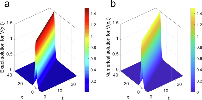
3D surfaces sketching a single travelling wave for exact and numerical solutions of $V(x,t)$ . The plots also compare the characteristics between the two solutions.

Export to PPT

Close

Fig. 5

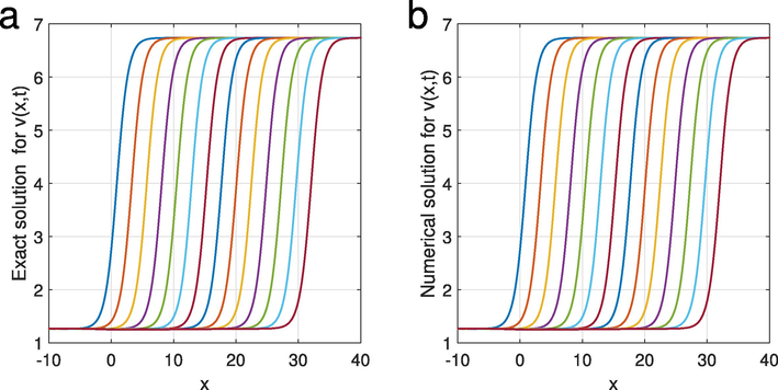
The time development for a solitary wave solution of the exact solution of $V(x,t)$ (left) and the numerical solution of $V(x,t)$ (right).

Export to PPT

Close

Fig. 6

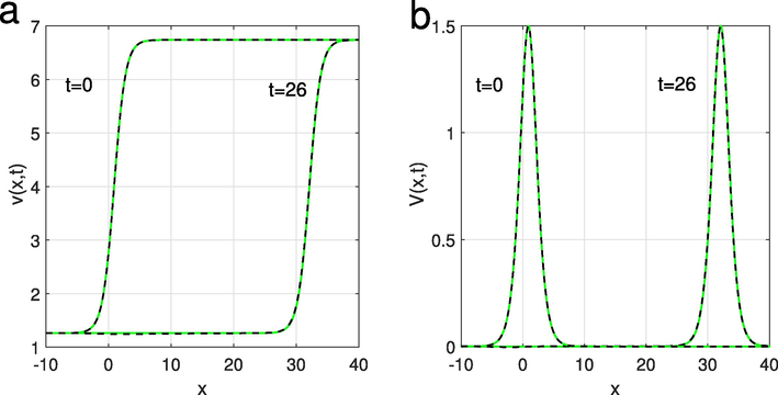
Diagram (a) shows that the exact solution of $v(x,t)$ is almost the same as its numerical solution while Figure (b) illustrates the behaviour of the exact and numerical solutions of $V(x,t)$ .

Export to PPT

6 Conclusion

The improved F-expansion approach combined with Riccati equation and the central finite differences have been utilized in this research to establish the exact travelling wave solutions and the numerical solutions, respectively, for Eqs. (12) and (13). The correctness of the accomplished solutions is verified by substituting the solutions into the leading equations. The numerical solutions approximately approach to the exact solutions for small $\mathrm{\Delta }x$ , as can be seen in Fig. 7. More precisely, $L_2$ error rapidly declines for smaller $\mathrm{\Delta }x$ , as presented in Table 1. The numerical scheme is found unconditionally stable via Von Neumann stability. Its accuracy is from second order in time and space. The applied processes lead to practical and powerful results. Eventually, we conclude that the employed techniques can be certainly used to deal with more complicated nonlinear evolution equations.

Declaration of Competing Interest

The authors declare that they have no known competing financial interests or personal relationships that could have appeared to influence the work reported in this paper.

References

- Benjamin-Feir-instability in nonlinear dispersive waves. Comput. Math. Appl.. 2012;64:3557-3568.
- [Google Scholar]
- Nonlinear dispersive Rayleigh-Taylor instabilities in magnetohydro-dynamic flows. Phys. Scr.. 2001;64:533-547.
- Nonlinear dispersive Kelvin-Helmholtz instabilities in magnetohydrodynamic flows. Phys. Scr.. 2003;67:340-349.
- Variational method for the nonlinear dynamics of an elliptic magnetic stagnation line. Eur. Phys. J. D. 2006;39:237-245.
- Calin Itu, Andreas Ochsner, Sorin Vlase, Marin Marin, 2019. Improved rigidity of composite circular plates through radial ribs. Proc. Inst. Mech. Eng. L J. Mater. Design Appl. 233(8), 1585–1593.
- Motion equation for a flexible one-dimensional element used in the dynamical analysis of a multibody system. Continuum Mech. Thermodyn. Contin. Mech. Thermodyn.. 2019;31(3):715-724.
- Praveen Agarwal, A., El-Sayed, A., Tariboon, J., 2021. Vieta-Fibonacci operational matrices for spectral solutions of variable-order fractional integro-differential equations. J. Comput. Appl. Math. 382, 113063.
- Study of hybrid orthonormal functions method for solving second kind fuzzy Fredholm integral equations. Adv. Differ. Equ.. 2020;2020(1):533.
- Growth of solutions for a coupled nonlinear Klein-Gordon system with strong damping, source, and distributed delay terms. Adv. Differ. Equ.. 2020;2020(1):335.
- Solvability of the boundary-value problem for a linear loaded integro-differential equation in an infinite three-dimensional domain. Chaos Solitons Fract.. 2020;140:110108
- Mustafa Inc, Mohammad Partohaghighi, Mehmet Ali Akinlar, Paraveen Agarwal, Yu-Ming Chu, 2020. New solutions of fractional-order Burger-Huxley equation. Results Phys. 18, 103290
- Construction of solitary wave solutions to the nonlinear modified Kortewege-de Vries dynamical equation in unmagnetized plasma via mathematical methods. Mod. Phys. Lett. A. 2018;33(32):1850183.
- Stability analysis of solitary wave solutions for the fourth-order nonlinear Boussinesq water wave equation. Appl. Math. Comput.. 2014;232:1094-1103.
- Yesim Glam Ozkan, Emrullah Yasar, Aly Seadawy, 2020. A third-order nonlinear Schrodinger equation: the exact solutions, group-invariant solutions and conservation laws. J. Taibah Univ. Sci. 14(1), 585–597
- Analytic approximate solutions for some nonlinear Parabolic dynamical wave equations. Taibah Univ. J. Sci.. 2020;14(1):346-358.
- Fundamental solutions for the coupled KdV system and its stability. Symmetry. 2020;12:429.
- Solving Frontier Problems of Physics: The Decomposition Method. Boston: Kluwer Academic Publishers; 1994.
- Application of Kudryashov method for the Ito equations. Appl. Appl. Math.. 2017;12(1):136-142.
- Constructions of the optical solitons and other solitons to the conformable fractional Zakharov-Kuznetsov equation with power law nonlinearity. J. Taibah Univ. Sci.. 2019;14(1):94-100.
- Analytical and numerical investigation for the DMBBM equation. CMES. 2020;122(2):743-756.
- Analytical and numerical investigation for Kadomtsev-Petviashvili equation arising in plasma physics. Phys. Scr.. 2020;95(4):045215
- The extended Jacobian elliptic function expansion approach to the generalized fifth order KdV equation. J. Phys. Math.. 2019;10(4):310.
- Numerical investigation of the Dispersive Long Wave Equation using an adaptive moving mesh method and its stability. Results Phys.. 2020;16:102870
- Riccati-Bernoulli Sub-ODE approach on the partial differential equations and applications. Int. J. Math. Comput. Sci.. 2020;15(1):367-388.
- Analytical and numerical solutions for the variant Boussinseq equations. J. Taibah Univ. Sci.. 2020;14(1):454-462.
- Using Krylov methods in the solution of large-scale differential- algebraic systems. SIAM J. Sci. Comput.. 1994;15:1467-1488.
- New traveling waves solutions to generalized Kaup-Kupershmidt and Ito equations. Appl. Math. Comput.. 2010;216:241-250.
- A class of exact periodic solutions of nonlinear envelope equation. J. Math. Phys.. 1995;36:4125-4137.
- Link between solitary waves and projective Riccati equations. J. Phys. A Math.. 1992;25:5609-5623.
- Extended tanh-function method and its applications to nonlinear equations. Phys. Lett. A. 2000;277:212-218.
- Exploratory approach to explicit solution of nonlinear evolutions equations. Int. J. Theor. Phys.. 2000;39:207-222.
- Exact solutions for nonlinear integro-partial differential equations using the generalized Kudryashov method. J. Egypt. Math. Soc.. 2017;25:438-444.
- Islam, M.d., Khan, K., Akbar, M.A., 2014. Mastroberardino A. A note on improved F-expansion method combined with Riccati equation applied to nonlinear evolution equations. R. Soc. Open Sci. 1, 140038.
- An extension of nonlinear evolution equations of the KdV (mKdV) type to higher order. J. Phys. Soc. Jpn.. 1980;49(2):771-778.
- The tanh method: exact solutions of nonlinear evolution and wave equations. Phys. Scr.. 1996;54:563-568.
- Nonlinear wave solutions of the Kudryashov-Sinelshchikov dynamical equation in mixtures liquid-gas bubbles under the consideration of heat transfer and viscosity. J. Taibah Univ. Sci.. 2019;13(1):1060-1072.
- The nonlinear integro-differential Ito dynamical equation via three modified mathematical methods and its analytical solutions. Open Phys.. 2020;18:24-32.
- Resolution of coincident factors in altering the flow dynamics of an MHD elastoviscous fluid past an unbounded upright channel. J. Taibah Univ. Sci.. 2019;13(1):1022-1034.
- Partial Differential Equations: Method and Applications. Netherlands: Taylor and Francis; 2002.
- A sine-cosine method for handling nonlinear wave equations. Math. Comput. Model.. 2004;40:499-508.
- The tanh method for travelling wave solutions of nonlinear equations. Appl. Math. Comput.. 2004;154:714-723.
- Exact solutions to the double sinh-Gordon equation by the tanh method and a variable separated ODE method. Comput. Math. Appl.. 2005;50:1685-1696.
- The extended tanh method for abundant solitary wave solutions of nonlinear wave equations. Appl. Math. Comput.. 2007;187:1131-1142.
- Zayed, E.M.E., Abourabia, A.M., Gepreel, K.A., 2006. Horbaty MM. On the rational solitary wave solutions for the nonlinear HirotaCSatsuma coupled KdV system. Appl. Anal. 85, 751–768
- The EHTA for nonlinear evolution equations. Appl. Math. Comput.. 2010;217:4306-4310.