

Translate this page into:
Some exact solutions of the Yu–Toda–Sasa–Fukuyama equation with time-dependent coefficients via two different methods
⁎Corresponding authors. haalmusawa@jazanu.edu.sa (Hassan Almusawa), sachin1jan@yahoo.com (Sachin Kumar)
-
Received: ,
Accepted: ,
This article was originally published by Elsevier and was migrated to Scientific Scholar after the change of Publisher.
Peer review under responsibility of King Saud University.
Abstract
In the current study, the generalized -expansion method and a new modified simple equation method (NMSEM) have been utilized to secure the exact solutions of the Yu-Toda-Sasa-Fukuyama (YTSF) equation with time-dependent coefficients, which describes two layers of liquid (or in an elastic) media. By implementing these methods, we have secured the three different families of travelling wave solutions (such as hyperbolic, rational and trigonometric functions) of the independent variables and the arbitrary parameters of the equation. Further, the graphical representation of the solitons are done with the help of the software Maple.
Keywords
Two layer liquid
(3+1)-dimensional YTSF
Travelling wave solution
Exact solutions

1 Introduction
Several complex phenomena in applied sciences and engineerings, such as plasma physics, quantum field theory, fluid dynamics, optics, optical fibres communication, and elastic media, are represented mathematically by nonlinear evolution equations (NLEEs). Such equations are the nonlinear Schrödinger equation, the Korteweg–de Vries equation, the Zakharov-Kuznetsov equation, the Boussinesq equation, and the Kadomtsev–Petviashvili equation (Ak et al., 2020; Biswas et al., 2020; Jyoti and Kumar, 2020; Kumar and Malik, 2022; Kumar et al., 2012; Malik et al., 2021; Ma, 2002; Ma, 2020; Nisar et al., 2022; Shumaila et al., 2021; Wang et al., 2021; Wazwaz, 2008). The exact solutions of these NLEEs perform a significant role in investigating different real-world phenomena and dynamical processes in several scientific disciplines. In the current scenario, various methods have been developed to secure the analytical solutions of these NLEEs, like the Hirota bilinear approach (Rizvi et al., 2020; Wazwaz, 2016), Bäcklund transform method (Rogers and Shadwick, 1982), inverse scattering transform (Ablowitz et al., 1991), Kudryashov scheme (Malik et al., 2021), Riccati equation method (Esen et al., 2022; Yıldırım et al., 2020), homogeneous balance method (Fan and Zhang, 1998), semi-inverse variational principle (Biswas et al., 2017; Kohl et al., 2020), modified extended tanh-method (El-Wakil and Abdou, 2007; Nuruddeen et al., 2020), Lie symmetry analysis (Kumar et al., 2020; Malik et al., 2021) and many more. Along with these methods, generalized
-expansion scheme (Wang et al., 2008; Zhang et al., 2008) and NMSEM (Irshad et al., 2017) gain attention of the many researcher. In the generalized
-expansion scheme, we utilized the basic knowledge of solutions of a second-order linear ordinary differential equation
, which produces the solutions in the form of hyperbolic, rational, and trigonometric functions. We didn’t use any widely accepted fundamental equations in the NMSEM. As a result, it is impossible to predict, based on prior experience, what kinds of solutions can be obtained using this strategy. This is the uniqueness and attractiveness of the NMSEM approach. The current study explores the YTSF equation with time-dependent coefficients, which describes the elastic quasi plane wave in a lattice or interfacial wave in a two-layer liquid
The remainder of the study is organized as follows: The generalized -expansion method and NMSEM are described in Sec. (2). In Sec. (3), the suggested approaches are used to find exact solutions to the (3 + 1)-dimensional YTSF equation with time-dependent coefficients. Sec. (4) shows some graphic representations of some solutions that have been found. Finally, the conclusion is presented.
2 Methods and their ideas
This section describes the generalized (
)-expansion method and the NMSEM, both of which are used to generate exact solutions to NLEEs. For this, consider the following NLEE
2.1 The Generalized -Expansion Method:
The following are the major steps in the generalized ( )-expansion scheme:
Step 1: Assume the solution of Eq. (2) can be stated as a polynomial in (
) as follows:
Step 2: Now the positive integer mis evaluated by applying the homogeneous balance between the highest order derivative and nonlinear terms of uin Eq. (2), which helps us to determine uexplicitly.
Step 3: Putting Eq. (3) and Eq. (4) into Eq. (2), and gathering up all terms of the same order of together, the Eq. (2) is transferred into a polynomial in . Then, for and , we construct a set of over-determined partial differential equations by setting each coefficient of this polynomial to zero.
Step 4: By solving the system of partial differential equations obtained in the previous step, the expressions for
and
can be found. Thus the solutions of Eq. (2) can be achieved based on the general solution of (4) and demonstrated as in the form of
, which is further dependent on the sign of the determinant
as follows:
2.2 The new modified simple equation method
The next steps will outline the essence of the NMSEM.
Step 1: Suppose that Eq. (2) has solution in the form of
Step 2: Now balance the highest-order derivatives and nonlinear terms in Eq. (2), to find the positive integer N.
Step 3: Calculate the necessary derivatives ,…of the unknown function and replace them in Eq. (2). As a result, a polynomial of can be obtained.
Step 4: From the obtained polynomial, now we gather all the terms of same power and by equating all these coefficients equal to zero, we yields a system of algebraic equations which can be solved to find and . As an outcome, we have the exact solutions of Eq. (2).
3 Application of proposed methods to the YTSF equation with time-dependent coefficients
In this section, we have derived the several exact solutions of the YTSF Eq. (1) by utilized the methods described in the above section. To overcome with the integral part in Eq. (1), we use the transformation
and then by integrating Eq. (1) w.r.t. xwith integral constant zero, we have
3.1 Application of the ( )-expansion method
According to the method described in the previous section, by applying the balance principle, we have
. Thus the solution of Eq. (7) can be written as:
Case 1: When
, the solution of Eq. (7) is given as
Case 2: When
, the solution of Eq. (7) is given as:
Case 3: When
, the solution of Eq. (7) is given as
3.2 Application of NMSEM
According to the method described in previous section, from Eq. (7), the positive integer Nis determined by classical balance procedure as
. Thus the solution of Eq. (7) according to Eq. (6) can be written as:
Case 1:
Case 2:
Case 3:
Case 4:
4 Graphical representation
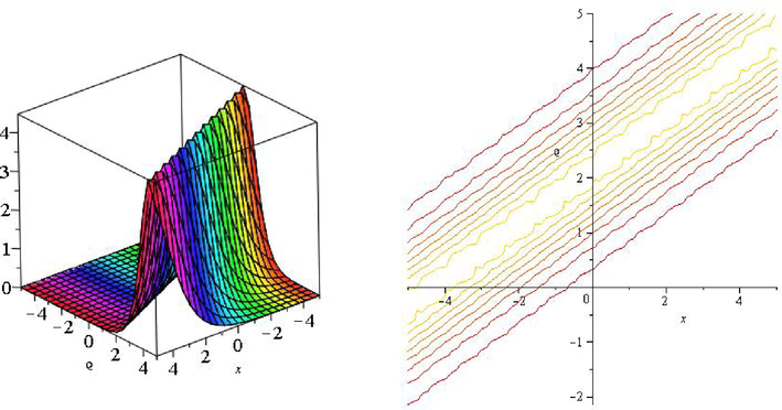
The physical interpretation of the solution of nonlinear differential equation can be done by its graphical representation, hence is important to be given. Fig. 1 demonstrate the solution Eq. (12) against xand
axis, at the points
, which shows the periodic solution. Fig. 2 represents the solution Eq. (14) against xand
axis, at the points
. Fig. 3 demonstrate the solution Eq. (16) against xand
axis, at the points
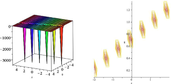
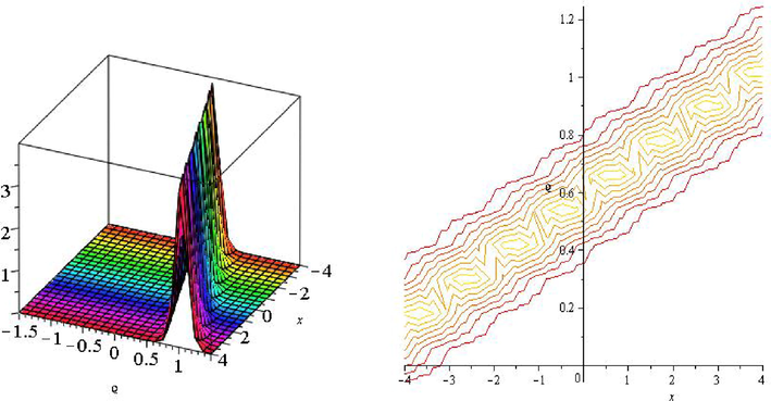
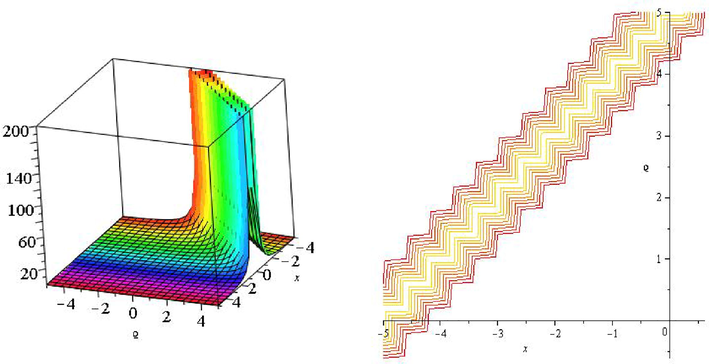
. Similarly, we have shown the graphical representation of solutions Eq. (21), Eq. (24), Eq. (27) and Eq. (30) as Fig. 4-Fig. 7, respectively. The Fig. 5 and Fig. 7 represent the bright wave solutions, while the other figures represents the periodical solutions. (See Fig. 6).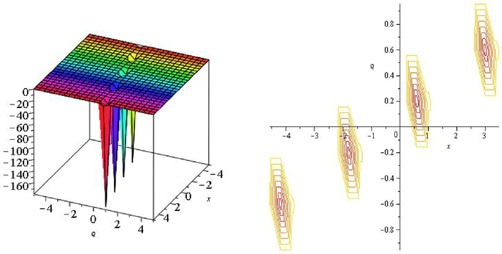
3D and contour plot of Eq. (12).
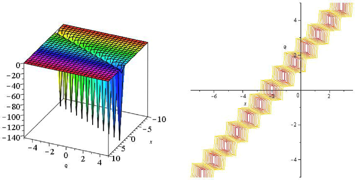
3D and contour plot of Eq. (14).
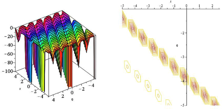
3D and contour plot of Eq. (16).
3D and contour plot of Eq. (21).
3D and contour plot of Eq. (30).
3D and contour plot of Eq. (24).
3D and contour plot of Eq. (27).
5 Conclusion
In this paper, we observed that the generalized -expansion method and NMSEM are convenient tools to obtain the solutions of the nonlinear (3 + 1)-dimensional YTSF equation. We study this equation with time-dependent coefficients, as in the real world phenomena, coefficients of nonlinear evolution equations vary with time and space. As a result, the exact solution of the variable coefficient nonlinear evolution equations has a broader range of applications. The obtained solutions can be divided into three families of the hyperbolic, rational and trigonometric functions, including independent variables and arbitrary parameters. Some solutions are represented graphically by giving particular values to the arbitrary constants and arbitrary parameters. Using these elementary and concise methods, namely the generalized -expansion approach and NMSEM, many nonlinear evolution equations of mathematical physics and other applied sciences can be solved efficiently. In the future, we will try to study the (3 + 1)-dimensional YTSF equation with time-dependent coefficients with the help of Lie symmetry analysis and derive some invariant and soliton solutions.
Acknowledgment
The author, Sandeep Malik, thankfully acknowledges CSIR SRF grant: 09/1051(0028)/2018-EMR-I. The author Sachin Kumar wants to acknowledge the financial support provided under the Scheme ‘Fund for Improvement of S & T Infrastructure (FIST)’ of the Department of Science & Technology (DST), Government of India, as evidenced by letter number: SR/FST/MS-I/2021/104 to the Department of Mathematics and Statistics, Central University of Punjab.
Declaration of Competing Interest
The authors declare that they have no known competing financial interests or personal relationships that could have appeared to influence the work reported in this paper.
References
- Mixed-type soliton propagations in two-layer-liquid (or in an elastic) medium with dispersive waveguides. J. Mol. Liq.. 2017;241:870-874.
- [Google Scholar]
- Solitons, nonlinear evolution equations and inverse scattering. Vol vol. 149. Cambridge University Press; 1991.
- Investigation of Coriolis effect on oceanic flows and its bifurcation via geophysical Korteweg–de Vries equation. Numer. Methods Partial Differ. Equ.. 2020;36(6):1234-1253.
- [Google Scholar]
- Conservation laws for optical solitons with polynomial and triple-power laws of refractive index. Optik: Int. J. Light Electron Optics. 2020;202:163476
- [Google Scholar]
- Optical soliton perturbation with anti-cubic nonlinearity by semi-inverse variational principle. Optik: Int. J. Light Electron Optics. 2017;143:131-134.
- [Google Scholar]
- New exact travelling wave solutions using modified extended tanh-function method. Chaos Solit. Fractals. 2007;31(4):840-852.
- [Google Scholar]
- Analytical soliton solutions of the higher order cubic-quintic nonlinear Schrödinger equation and the influence of the model’s parameters. J. Appl. Phys.. 2022;132(5):053103
- [Google Scholar]
- A new modification in simple equation method and its applications on nonlinear equations of physical nature. Results Phys.. 2017;7:4232-4240.
- [Google Scholar]
- Exact non-static solutions of Einstein vacuum field equations. Chin. J. Phy.. 2020;68:735-744.
- [Google Scholar]
- Sequel to highly dispersive optical soliton perturbation with cubic-quintic-septic refractive index by semi-inverse variational principle. Optik: Int. J. Light Electron Optics. 2020;203:163451
- [Google Scholar]
- Optical solitons with Kudryashov’s equation by Lie symmetry analysis. Phys. Wave Phenom.. 2020;28(3):299-304.
- [Google Scholar]
- The (3+1)-dimensional Benjamin-Ono equation: Painlevé analysis, rogue waves, breather waves and soliton solutions. Int. J. Mod. Phys. B. 2022;36(20):2250119.
- [Google Scholar]
- Painlevé analysis, Lie symmetries and exact solutions for (2+1)-dimensional variable coefficients Broer-Kaup equations. Commun. Nonlinear Sci. Numer. Simul.. 2012;17(4):1529-1541.
- [Google Scholar]
- A (2+1)-dimensional Kadomtsev-Petviashvili equation with competing dispersion effect: Painlevé analysis, dynamical behavior and invariant solutions. Results Phys.. 2021;23:104043
- [Google Scholar]
- Optical solitons and bifurcation analysis in fiber Bragg gratings with Lie symmetry and Kudryashov’s approach. Nonlinear Dyn.. 2021;105(1):735-751.
- [Google Scholar]
- Different analytical approaches for finding novel optical solitons with generalized third-order nonlinear Schrödinger equation. Results Phys.. 2021;29:104755
- [Google Scholar]
- Complexiton solutions to the Korteweg-de Vries equation. Phys. Lett. A. 2002;301(1–2):35-44.
- [Google Scholar]
- N-soliton solutions and the Hirota conditions in (2+1)-dimensions. Opt. Quantum Electron.. 2020;52(12):511.
- [Google Scholar]
- New soliton solutions of Heisenberg ferromagnetic spin chain model. Pramana. 2022;96(1):28.
- [Google Scholar]
- Investigating the tangent dispersive solitary wave solutions to the equal width and regularized long wave equations. J. King Saud Univ.-Sci.. 2020;32(1):677-681.
- [Google Scholar]
- Lump and rogue wave solutions for the Broer-Kaup-Kupershmidt system. Chin. J. Phys.. 2020;68:19-27.
- [Google Scholar]
- Bäcklund transformations and their applications. Academic Press; 1982.
- Soliton solutions of nonlinear Boussinesq models using the exponential function technique. Phys. Scr.. 2021;96(10):105209
- [Google Scholar]
- Bright soliton solutions of the (2+1)-dimensional generalized coupled nonlinear Schrödinger equation with the four-wave mixing term. Nonlinear Dyn.. 2021;104(3):2613-2620.
- [Google Scholar]
- The -expansion method and travelling wave solutions of nonlinear evolution equations in mathematical physics. Phys. Lett. A. 2008;372(4):417-423.
- [Google Scholar]
- The extended tanh method for the Zakharov-Kuznetsov (ZK) equation, the modified ZK equation, and its generalized forms. Commun. Nonlinear Sci. Numer. Simul.. 2008;13(6):1039-1047.
- [Google Scholar]
- The simplified Hirota’s method for studying three extended higher-order KdV-type equations. J. Ocean Eng. Sci.. 2016;1(3):181-185.
- [Google Scholar]
- Analyzing the combined multi-waves polynomial solutions in a two-layer-liquid medium. Comput. Math. with Appl.. 2018;76(2):276-283.
- [Google Scholar]
- Optical solitons with Kudryashov’s model by a range of integration norms. Chin. J. Phys.. 2020;66:660-672.
- [Google Scholar]
- A generalized -expansion method and its applications. Phys. Lett. A. 2008;372(20):3653-3658.
- [Google Scholar]


